Colorizing Old Russian Photographs... Automatically!
TLDR
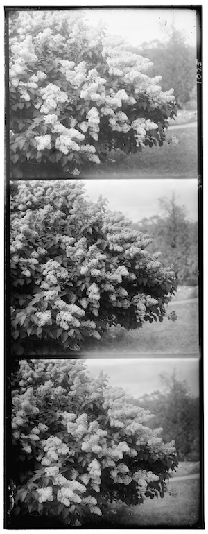
I implemented, from scratch, an image colorization algorithm that can turn this:
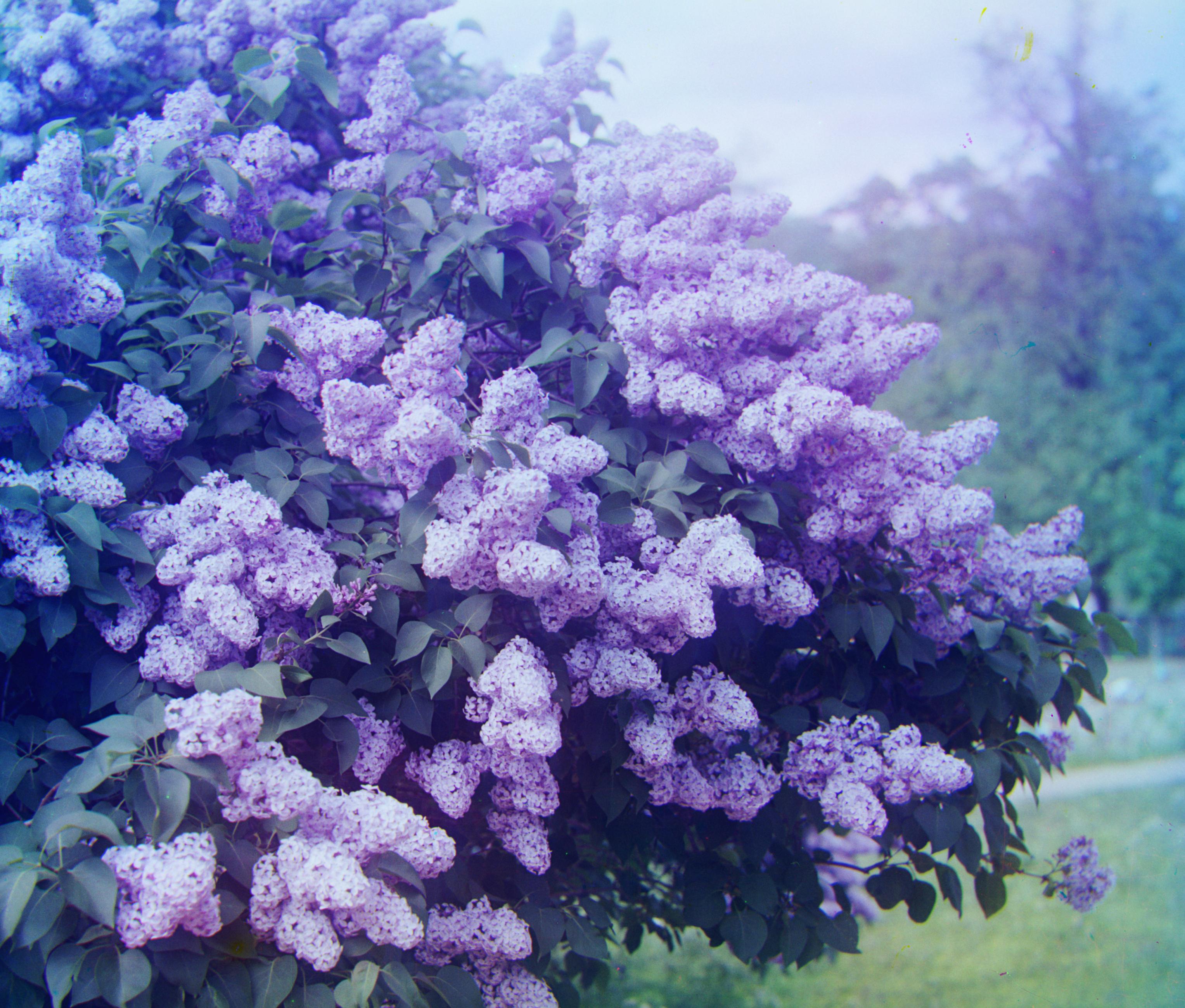
Into this:
Part 0: Background Information
This Fall 2025 semester, I’m taking a computer vision class, titled CS 180, taught by Professors Alexei Efros and Angjoo Kanazawa at UC Berkeley. The first assignment is to colorize some images from the Prokudin-Gorskii photo collection, an example of which you saw above. Basically, the photographer took three exposures of every scene onto a glass plate using blue, green, and red filters. The “blue” image is the one on the top, the “green” the one in the middle, and the “red” the one at the bottom.
Our task is to turn the stack of three grayscale images into a single color image.
Part 1: Single-Scale Colorization
The first approach you might try is to naively divide the image into three. Take this image for example:
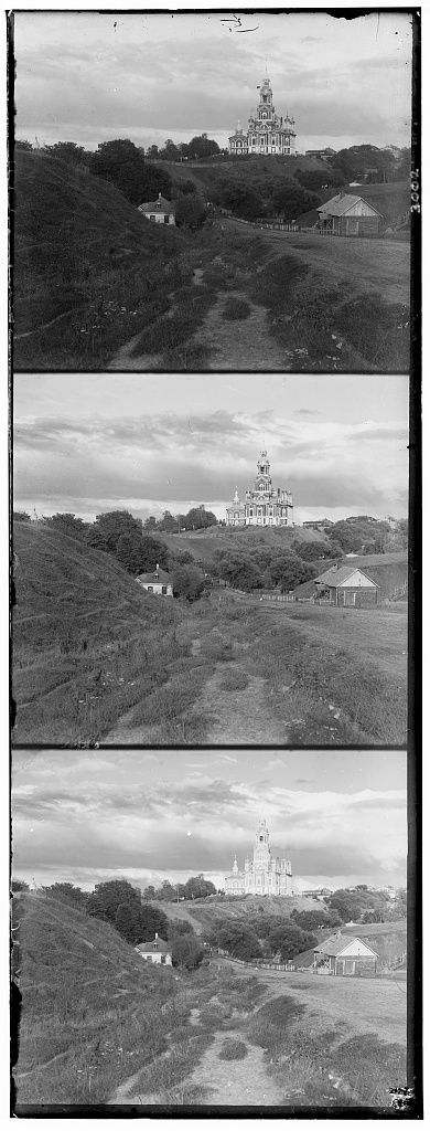
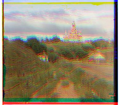
If we naively stack the three thirds of the image on top of each other, here’s what you end up with:
We need a better approach - a way to somehow align the three channels. That is, we want to find translation (dx, dy) to apply to the green and red channels such that they differ as little as possible from the blue image.
Translation Scoring Metric
There are many ways you can measure the “best translation” between two images.
I used the Normalized Cross-Correlation (NCC) metric: I flatten both images into 1-D column vectors, then normalize them and compute their dot product. In pseudocode, we want to find: dot_product(image1./||image1|| , image2./||image2||).
The higher the resulting dot product, the better the match between the two images.
Another option is to use the L2 norm, which can deliver reasonably good results as well. However, the assignment instructions recommended NCC, and I found that it worked well for me.
Translation Search Algorithm
Now that we know how to measure a good displacement, how can we actually calculate which displacement is optimal? One idea is to brute-force try all possible translations within a particular range: I used the interval [-15, 15]. This algorithm1 is reasonably performant, but it had a problem: it was too slow, taking upwards of 50 seconds for some images. We can do better by being smarter about where we search.
Instead of checking every possible displacement, I start with a larger step size to get a rough estimate, and then progressively refine the search with smaller step sizes until I get to pixel-level accuracy. This way, we quickly narrow down the promising areas of the search space.
For example, let’s say that we set the max number of search steps to 4: I first try displacements in increments of 4 pixels. Once I find the best candidate, I reduce the step size to 2 and search in that neighborhood, and finally reduce the step size to 1 to lock in the exact displacement.
Here’s an example of what the algorithm does to a sample image. Notice how neatly aligned the channels are compared to before:
Part 2: Using an Image Pyramid
The single-scale approach we just discussed works well for lower-resolution JPEG images. But for higher-resolution TIFF images, we need a separate approach: the optimal displacement might be a lot more than 15 pixels in any direction. This is where the image pyramid comes in. Here’s how the image pyramid approach works:
- Build a pyramid for each channel by repeatedly downsampling by 2 for several levels. I found that having 5 levels worked well for me.
- Start at the coarsest level and align red/green to blue.
- Propagate the found displacement to the next level, scaling by 2. We scale by two because the new image has twice the resolution in both dimensions.
- Refine our estimation at the new level using the single-scale approach described earlier.
- Repeat until you reach the original resolution.
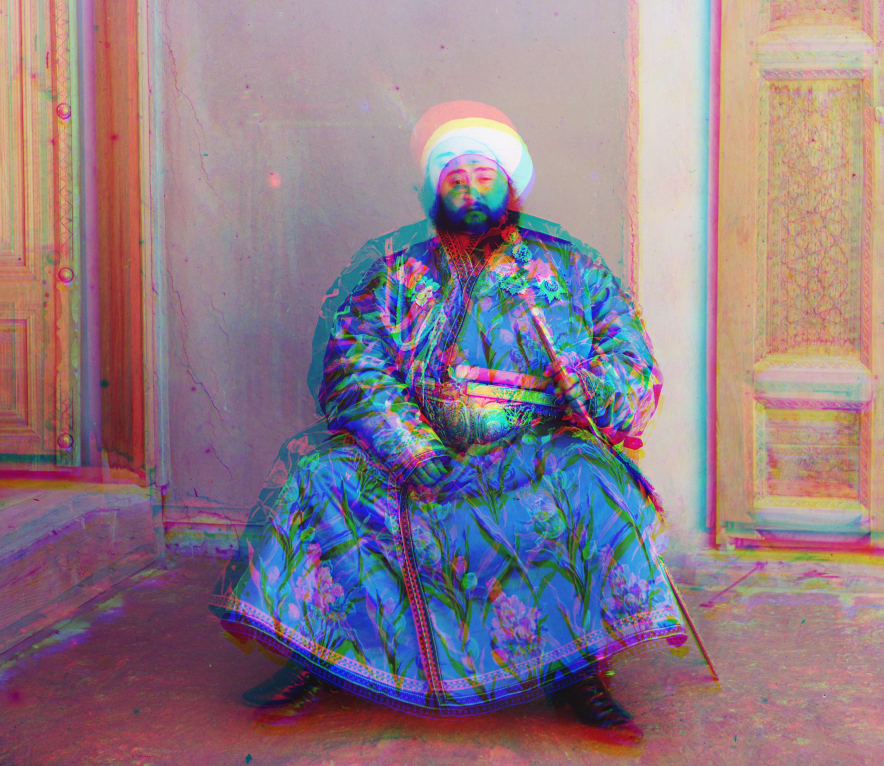
This drastically improves results for some images. For example, the Emir of Bukhara image below:
Without the pyramid, it looks like this:
Conversely, with the pyramid it looks much better:
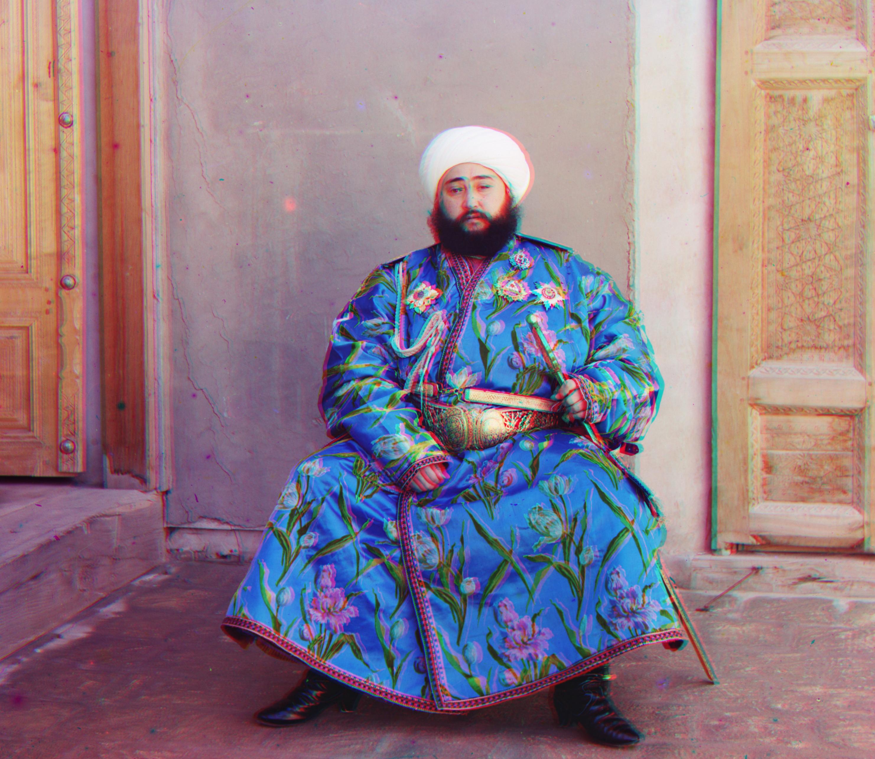
Getting the Emir of Bukhara image to align properly was a big challenge. I had to patiently tweak the pyramid levels and search range to get it right. Even then, my result isn’t perfect because the red channel’s brightness values are very different from those of the blue and green images. I think there is a limit to how good the reconstruction can be using just NCC and (x, y) translations. A more advanced technique like edge detection might be helpful here.
Misc. Implementation Details
- I crop 12.5% off the borders of the image before computing the NCC, as we don’t want border artifacts to influence the final alignment.
- As a post-processing step, I crop 10% off the borders of the final images; the borders of the image contain artifacts from color alignment and are not visually appealing.
- Resizing of images is done via
cv2.resizeas opposed to manually applying a Gaussian filter.
Gallery of Pyramid Results
Here are some of the best results I obtained using the image pyramid approach. My displacements are in the form (dx, dy).

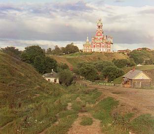
cathedral
Green channel offset: (2, 5) Red channel offset: (3, 12) |
church
Green channel offset: (4, 25) Red channel offset: (-4, 58) |
|
emir
Green channel offset: (24, 49) Red channel offset: (57, 103) |
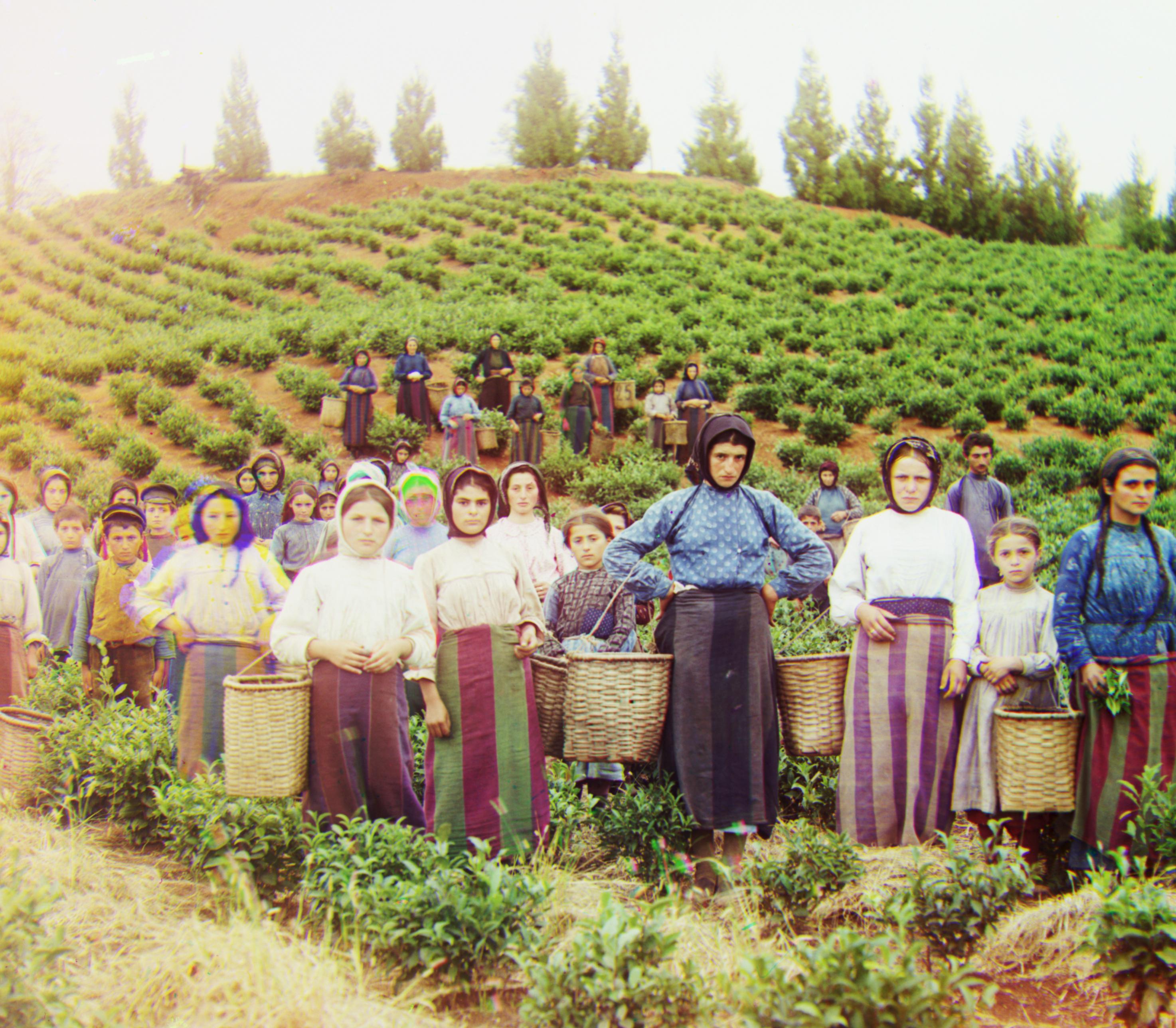
harvesters
Green channel offset: (17, 60) Red channel offset: (14, 124) |
|
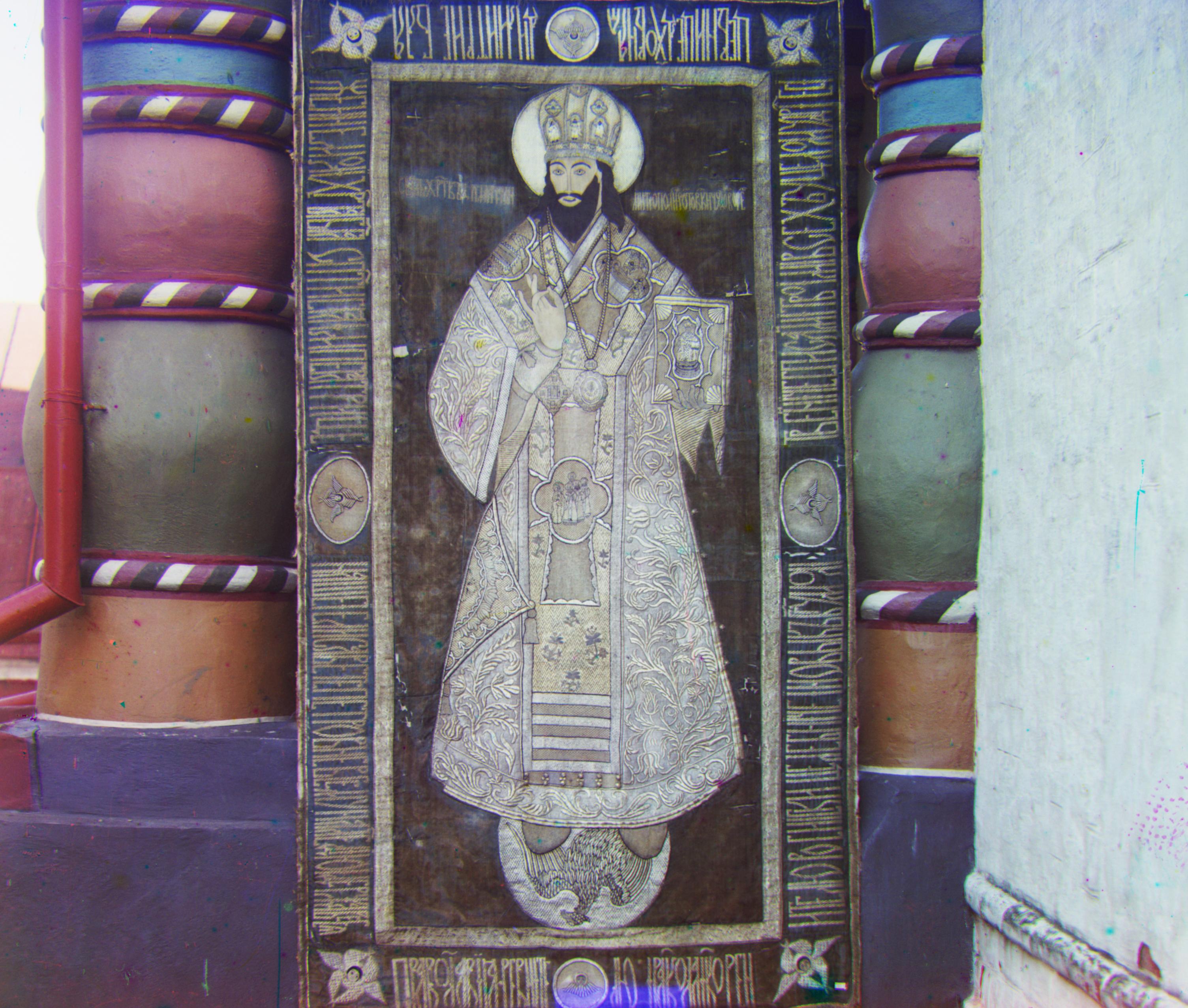
icon
Green channel offset: (17, 41) Red channel offset: (23, 89) |
italil
Green channel offset: (21, 38) Red channel offset: (35, 77) |
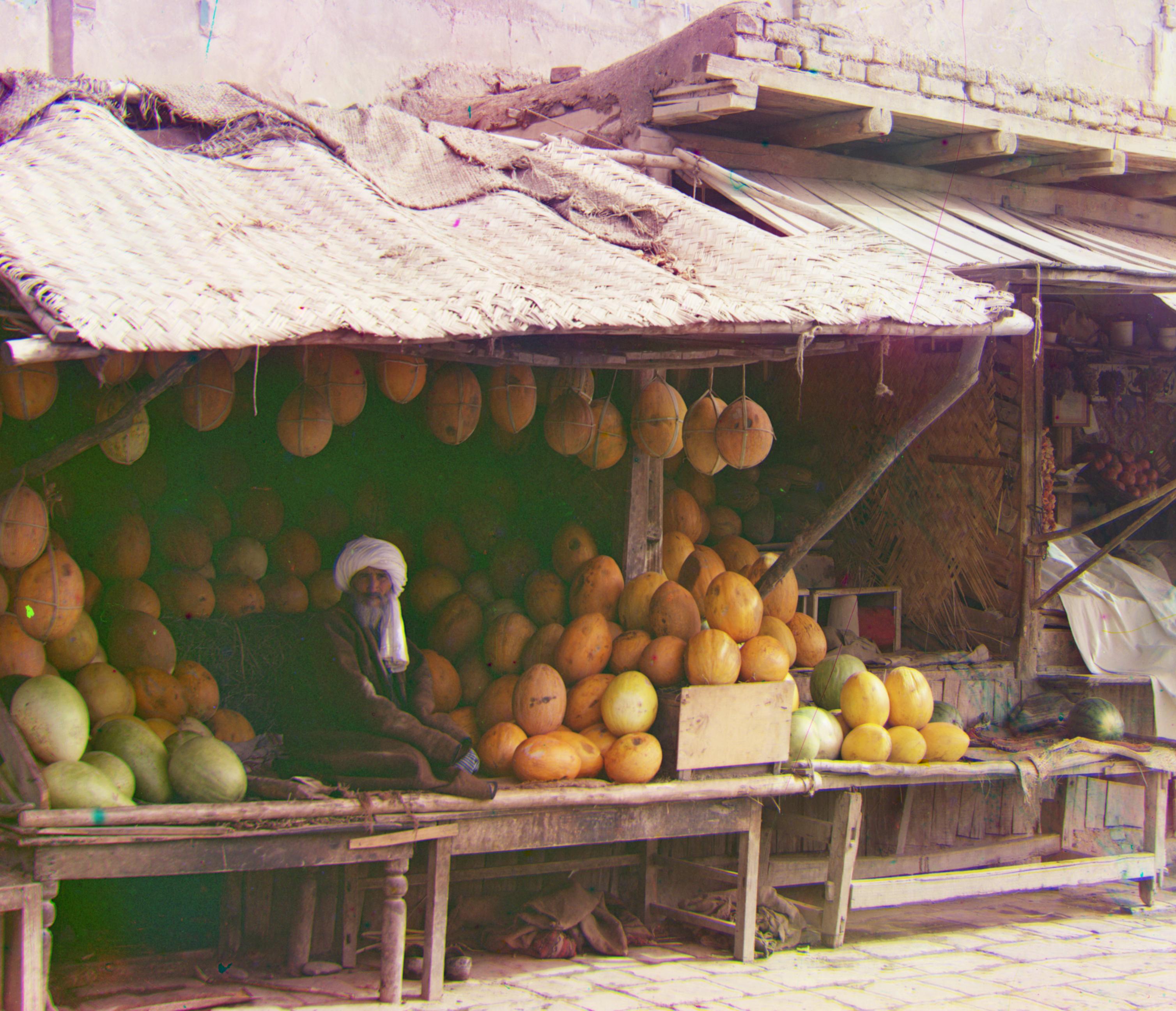
melons
Green channel offset: (10, 81) Red channel offset: (13, 178) |
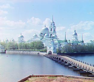
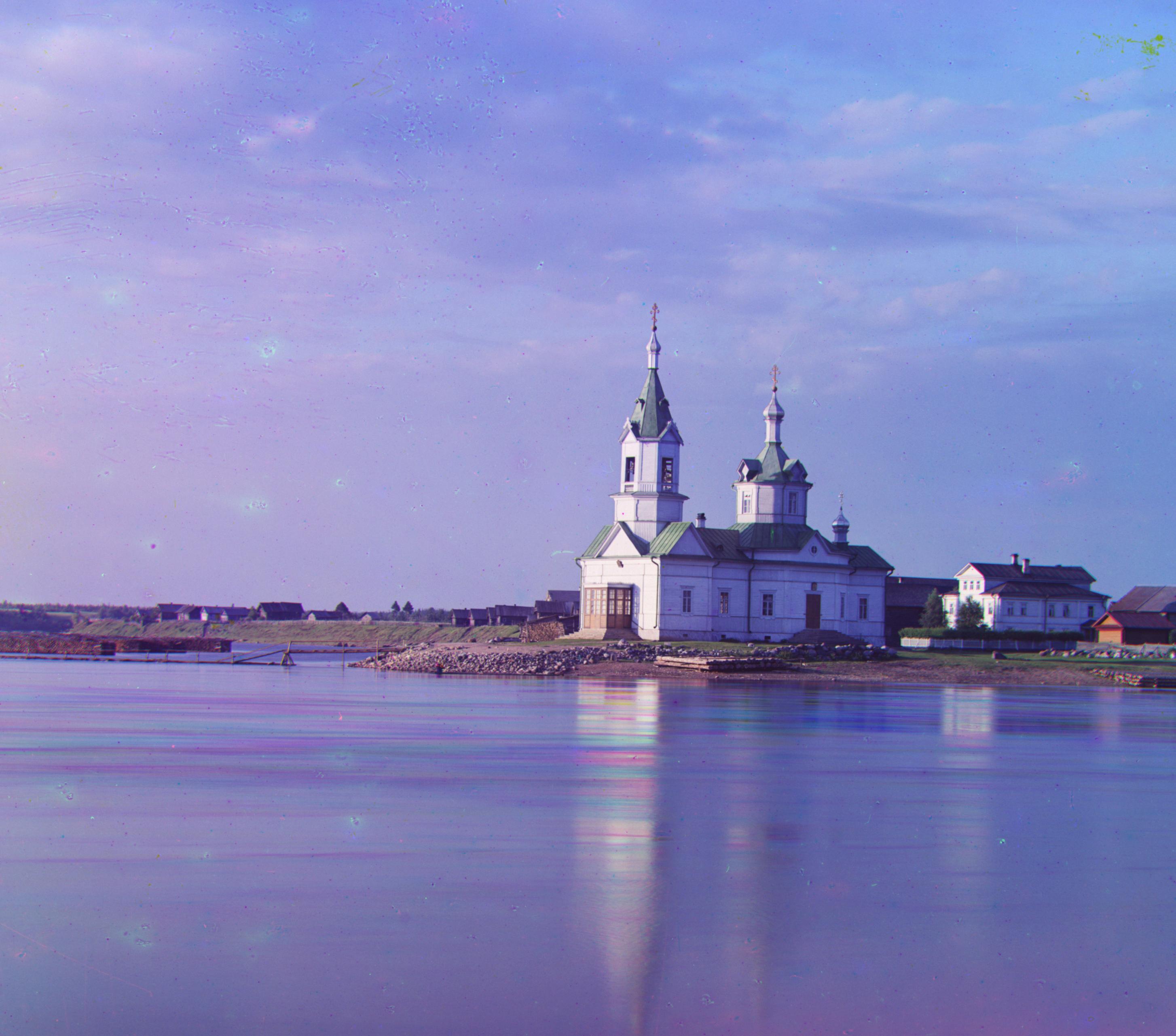
monastery
Green channel offset: (2, -3) Red channel offset: (2, 3) |

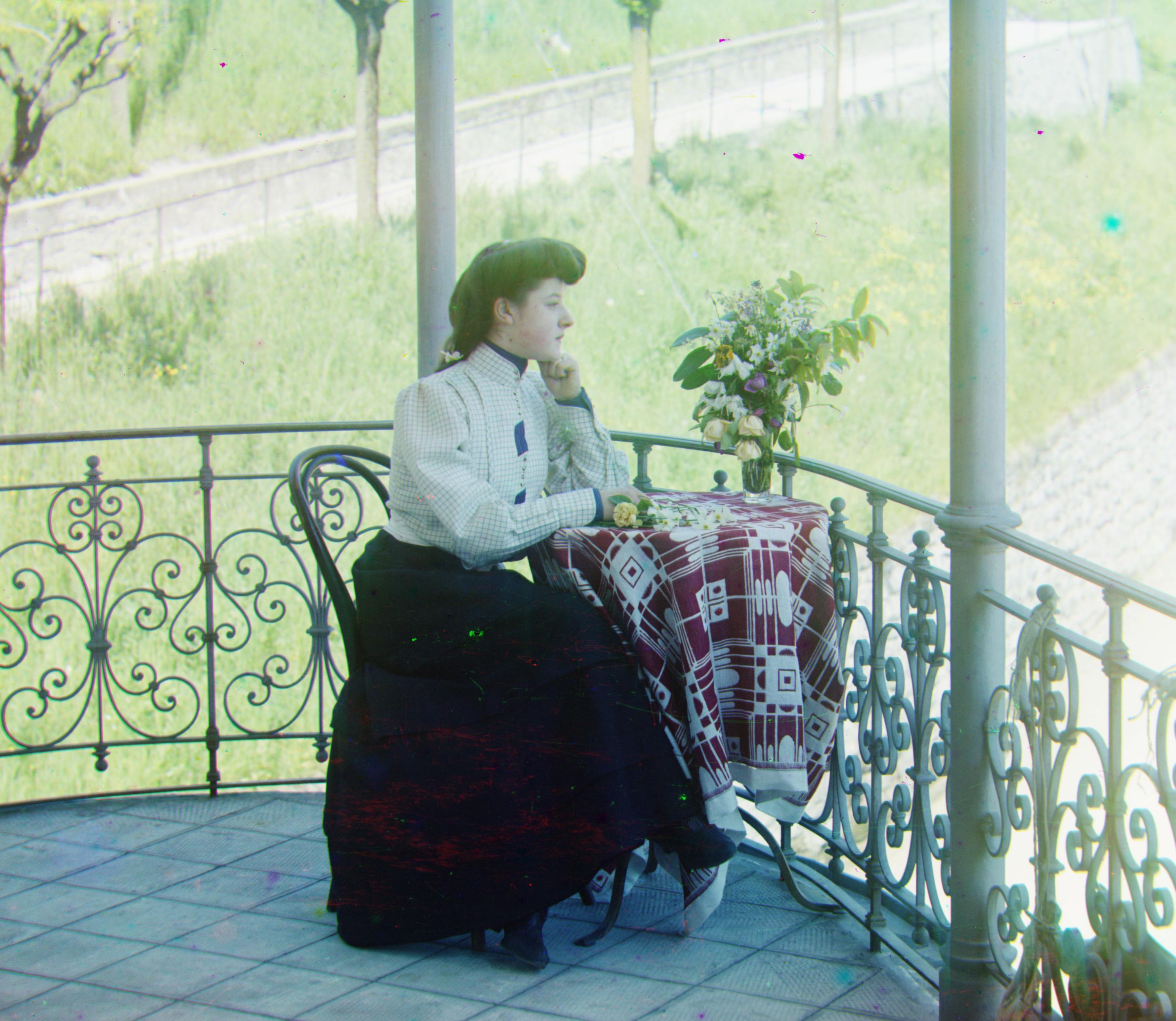
self_portrait
Green channel offset: (29, 79) Red channel offset: (37, 176) |
|
siren
Green channel offset: (-6, 49) Red channel offset: (-25, 96) |
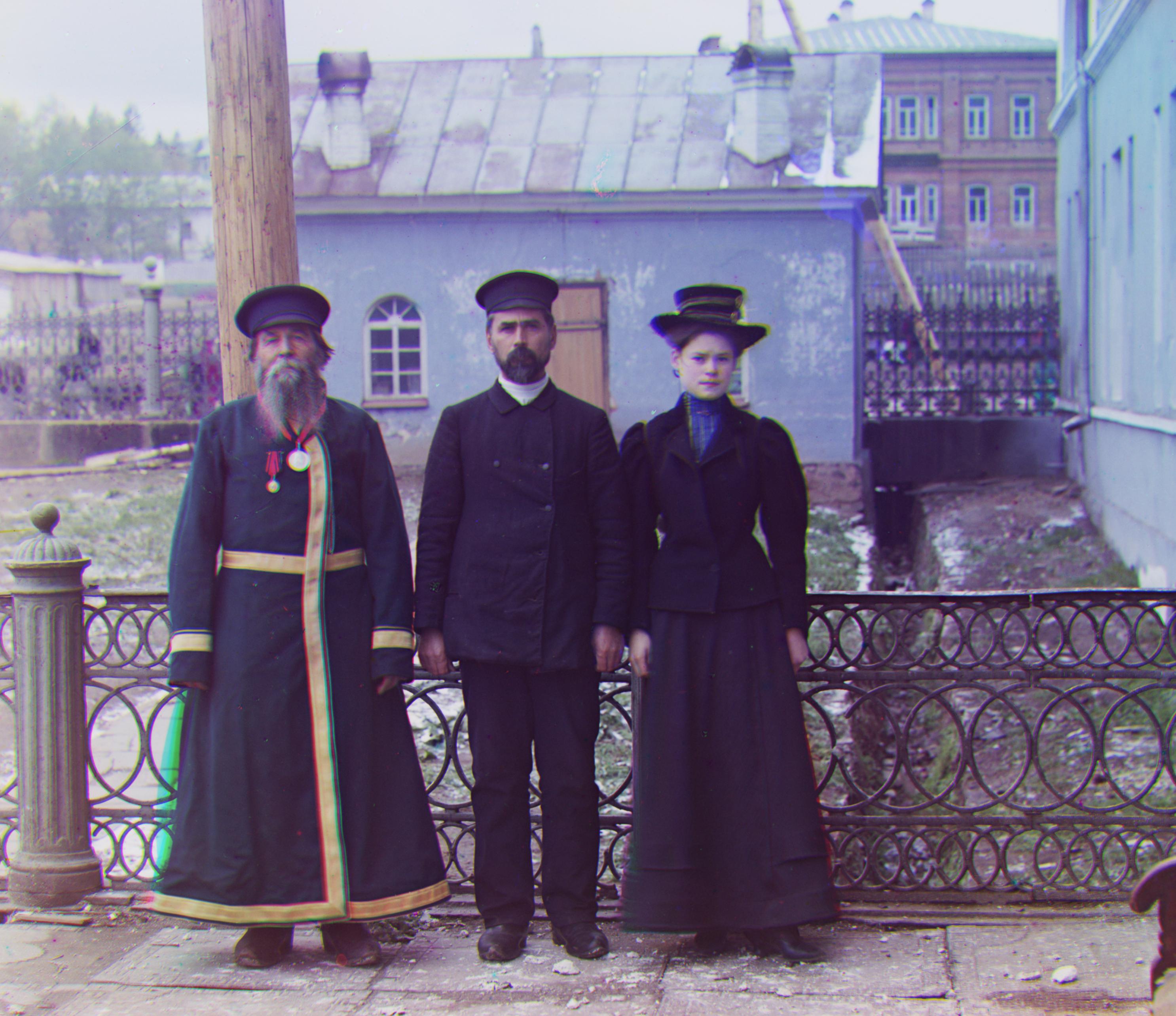
three_generations
Green channel offset: (14, 53) Red channel offset: (11, 111) |
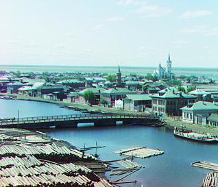
tobolsk
Green channel offset: (3, 3) Red channel offset: (3, 6) |
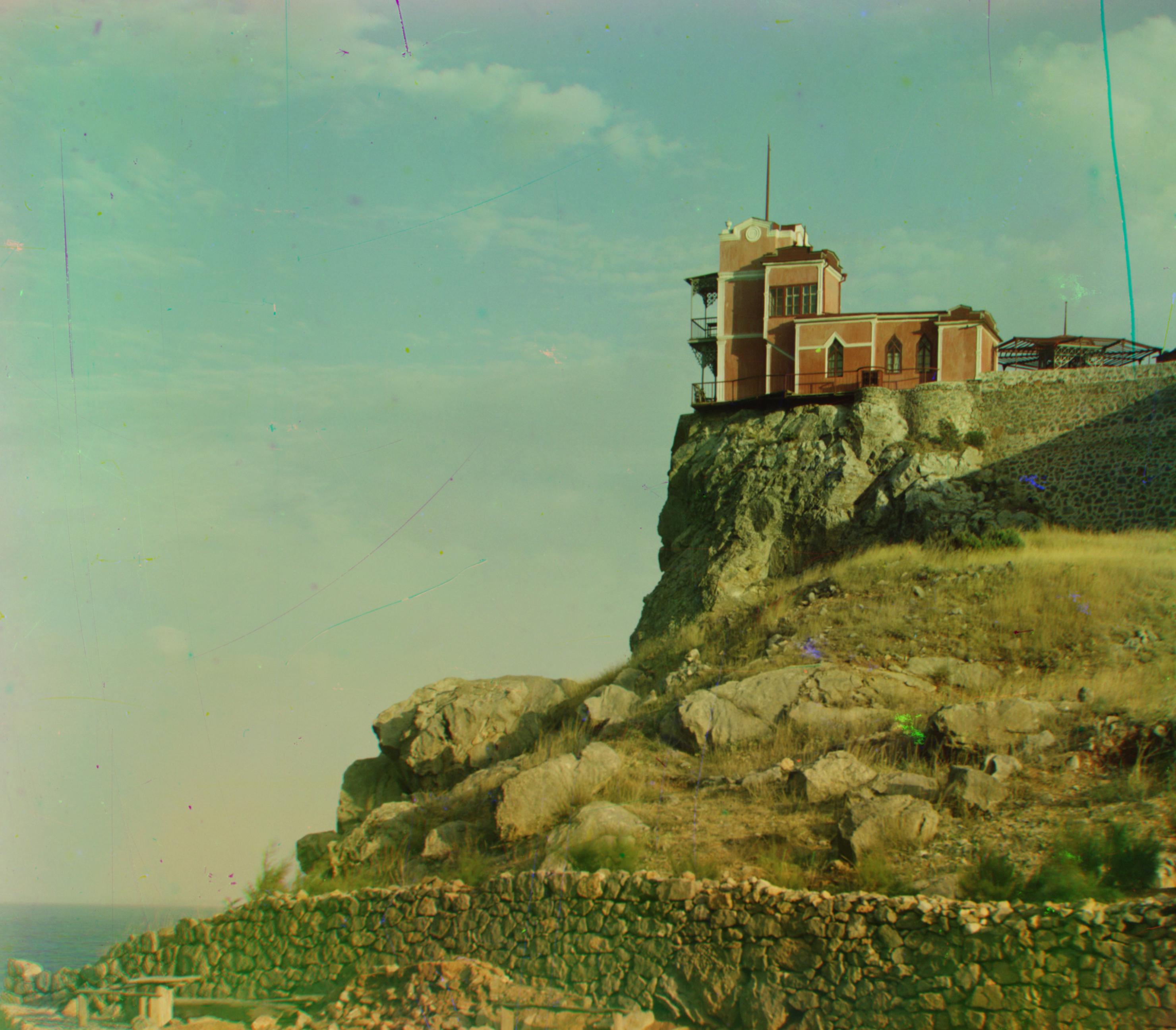
lastochikino
Green channel offset: (-2, -3) Red channel offset: (-9, 75) |
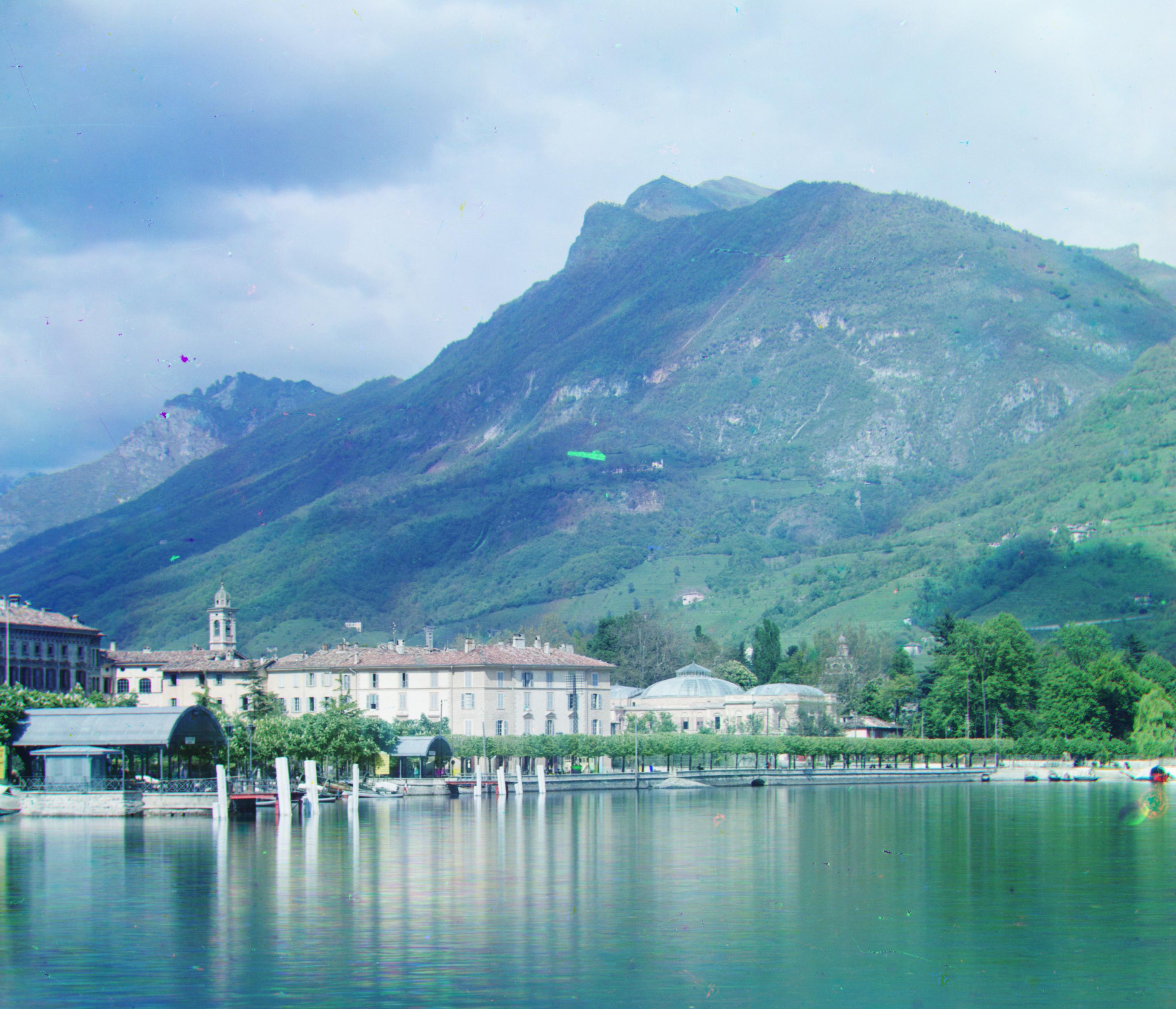
lugano
Green channel offset: (-16, 41) Red channel offset: (-29, 93) |
Gallery of Additional Images from the Prokudin-Gorskii Collection
I selected these additional images from the original collection to test my algorithm:
Green channel offset: (3, 29)
Red channel offset: (-7, 71) |
Green channel offset: (-12, 39)
Red channel offset: (-27, 86) |
Green channel offset: (-18, 66)
Red channel offset: (-34, 146) |
-
I don’t reproduce the code for this algorithm in this blog post, as per class policies. ↩