Diffusion Image Generation Models from Scratch in PyTorch

Table of Contents

• Part 0: Setup
• Part A: Sampling Loops
  • 1.1 Implementing the Forward Process
  • 1.2 Classical Denoising
  • 1.3 One-Step Denoising
  • 1.4 Iterative Denoising
  • 1.5 Diffusion Model Sampling
  • 1.6 Classifier-Free Guidance (CFG)
  • 1.7 Image-to-Image Translation
  • 1.8 Visual Anagrams
  • 1.9 Hybrid Images
• Part B: Flow Matching from Scratch!
  • 1. Single-Step Denoising UNet
  • 2. Training a Diffusion Model

TLDR

In this project, I explore techniques for sampling from pretrained diffusion models (Part A) and train my own class-conditioned flow matching model from scratch using a UNet (Part B).

Here’s an example of an image sampled from the model I trained in part B, which can generate images of any handwritten digit between 0 and 9:

Part 0: Setup

In this part, I experimented with the DeepFloyd IF diffusion model. This is a text-to-image model that operates in two stages:

1. Stage 1: Generates a 64x64 resolution image from the text prompt.
2. Stage 2: Upscales the image to 256x256 and adds details.

I generated images for three different prompts using 20 inference steps. The random seed used for all parts of this project is 100.

“An oil painting of a snowy mountain village”

“A photo of a cat”

“A photo of a temple”

The outputs here are pretty good in my opinion, which is a testament to the quality of Deepfloyd IF’s training process.

Comparison with More Inference Steps

I also generated the temple image with 100 inference steps. This lets us see if the quality improves with more denoising iterations.

The image turned out a little bit oversaturated, which makes me believe that more inference steps were not necessary, at least for this specific prompt. That said, it didn’t ruin the image either, so my conclusion is that the number of inference steps has to be chosen qualitatively and depends on the prompt and model being used.

Part 1: Sampling Loops

1.1 Implementing the Forward Process

The forward process in diffusion models adds noise to a clean image $x_0$ to produce a noisy image $x_t$ at timestep $t$. The process is defined by the equation:

Which allows us to sample $x_t$ directly:

Here are the results of the forward process on the Campanile image at different noise levels ($t \in {250, 500, 750}$):

1.2 Classical Denoising

I first attempted to remove the noise using classical Gaussian blurring. As expected, this simple technique fails to recover the details, blurring out both the noise and the high-frequency content of the image.

No amount of Gaussian blurring can bring back parts of the image that were already lost. We need something more sophisticated.

1.3 One-Step Denoising

Using a pretrained diffusion model, we can try to recover $x_0$ in a single step. The model is trained to estimate the noise $\epsilon$ in a noisy image $x_t$. Given the estimate $\epsilon_\theta(x_t, t)$, we can approximate $x_0$ by inverting the forward process equation:

The model does a much better job than Gaussian blur, but for high noise levels (t=750), the one-step reconstruction is blurry and lacks fine detail. This is because the initial assumption of mapping directly to $x_0$ is difficult when the signal is heavily corrupted.

1.4 Iterative Denoising

To get high-quality images, we denoise iteratively. Starting from pure noise or a noisy image, we repeatedly apply the update step:

which effectively steps from $t$ to $t’$ by removing a fraction of the predicted noise and adding new variance. In practice, we don’t iteratively denoise over all 1000 timesteps, as that would be too costly. Instead, we iterate over a strided subset of timesteps (for this assignment, I set the stride to 30)

Here is the progression of iterative denoising (using strided sampling):

Comparison:

The iterative result is significantly sharper than the one-step estimation.

1.5 Diffusion Model Sampling

We can generate new images by running the iterative denoising loop starting from pure Gaussian noise ($x_T \sim \mathcal{N}(0, \mathbf{I})$) with the prompt “a high quality photo”.

1.6 Classifier-Free Guidance (CFG)

To improve image quality and prompt adherence, I implemented Classifier-Free Guidance, also known as CFG. We compute two noise estimates: one conditional on the text prompt ($\epsilon_{cond}$) and one unconditional ($\epsilon_{uncond}$). The final noise estimate is:

where $\gamma > 1$ is the guidance scale. This pushes the image towards the prompt.

The generated images are sharper and more clearly defined compared to the unguided samples.

1.7 Image-to-Image Translation

By taking a real image, adding noise to it up to a certain timestep $t$, and then running the iterative denoising process from there, we can edit images. This allows us to balance maintaining the original structure (via the starting noisy image) and generating new details (via the denoising loop).

Below I show edits of the Campanile image at noise levels [1, 3, 5, 7, 10, 20] with the conditional text prompt “a high quality photo”. I also show two edits of my own test images, which are captioned “original” in the below image:

1.7.1 SDEdit

Artificial Image Transition (SDEdit):

Hand-Drawn Image Transition:

1.7.2 Inpainting

We can use a mask to keep parts of the image constant while denoising the rest. At each step of the backward process, we force the pixels outside the mask to match the noisy version of the original image, while letting the model hallucinate content inside the mask.

1.7.3 Text-Conditional Image-to-Image Translation

We can guide the SDEdit process with specific text prompts to change the style or content of the image. Results for all three images are below:

Here, the prompt was “a rainy day”. Notice now the images gradually have more and more “rain-like” features. For example, the campanile turns into a bolt of lightning for time step 5 of the first row. Similarly, the happy face drawing starts to show small droplets of rain on its sides.

1.8 Visual Anagrams

Visual anagrams are images that look like one thing when upright and another when flipped. I implemented this by averaging the noise estimates for two different prompts, one computed on the upright image and one on the flipped image:

1.9 Hybrid Images

Hybrid images combine the low frequencies of one image with the high frequencies of another. We can generate these with diffusion by combining noise estimates:

Part B: Flow Matching from Scratch!

In this part, we implement a diffusion model from scratch using the MNIST dataset. We start with a simple single-step denoiser and then move on to a full diffusion model with time conditioning. Unless otherwise stated, the random seed used for all subparts was 100.

1. Single-Step Denoising UNet

1.1 Architecture

The backbone of our denoiser is a UNet. At its core, a UNet is just an autoencoder with a twist: it compresses the image into a bottleneck to capture global context (like “this is a digit 8”) and then expands it back to the original size. The “twist” is the skip connections—wires that bypass the bottleneck and plug the detailed, high-resolution features from the encoder directly into the decoder. This lets the network reconstruct fine details (like edges and noise) that would otherwise be lost in compression.

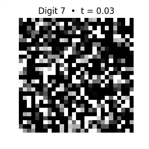
1.2 Noising Process Visualization

The noising process adds Gaussian noise to a clean image $x$. \(z = x + \sigma \epsilon, \quad \epsilon \sim \mathcal{N}(0, I)\)

Here is the effect of varying $\sigma$ on a clean image:

1.2.1 Training the Denoiser

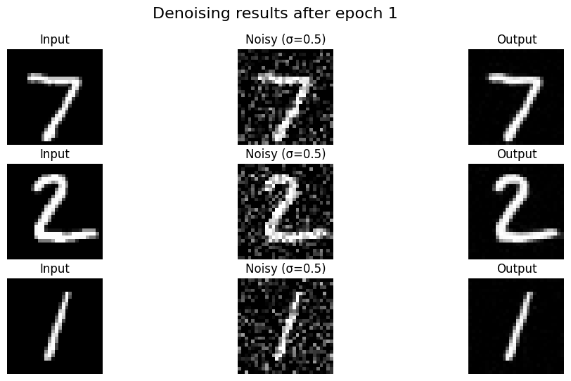
I trained a UNet to denoise images with $\sigma = 0.5$. The objective is to minimize the L2 distance between the denoised image and the original clean image: \(L = \mathbb{E}_{z,x} \|D_{\theta}(z) - x\|^2\)

Training Loss Curve:

Denoising Results (Epoch 1 vs Epoch 5): The model learns to remove the noise effectively after just a few epochs.

1.2.2 Out-of-Distribution Testing

The model was trained only on $\sigma=0.5$. Here I tested it on other noise levels. It performs reasonably well on lower noise levels but struggles when the noise level is much higher than what it was trained on (e.g., $\sigma=1.0$).

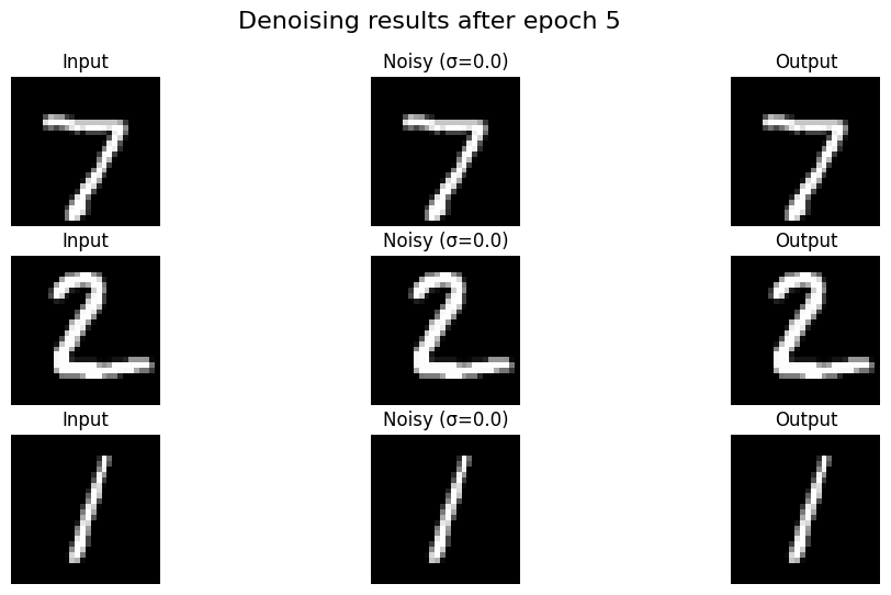$\sigma=0.0$	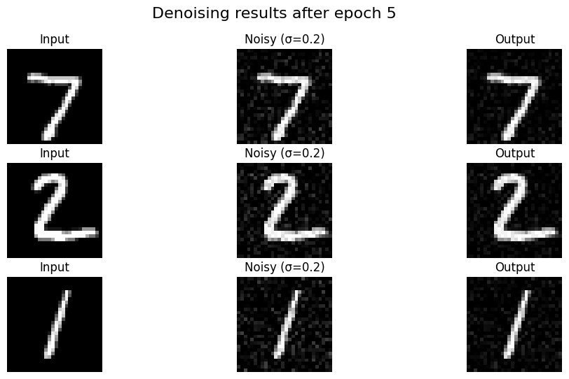$\sigma=0.2$
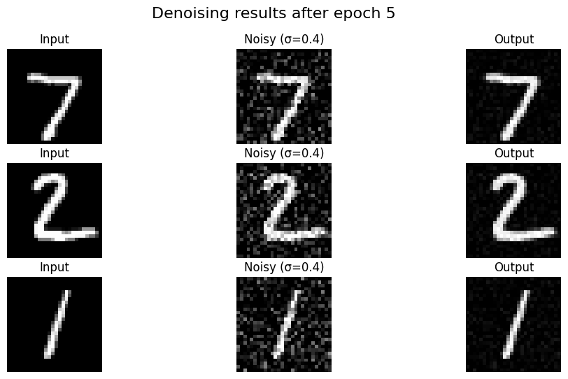$\sigma=0.4$	$\sigma=0.5$
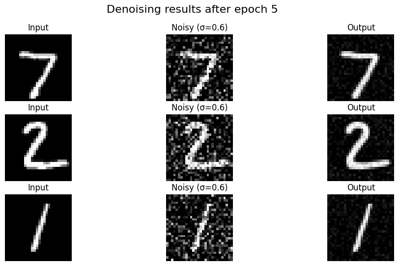$\sigma=0.6$	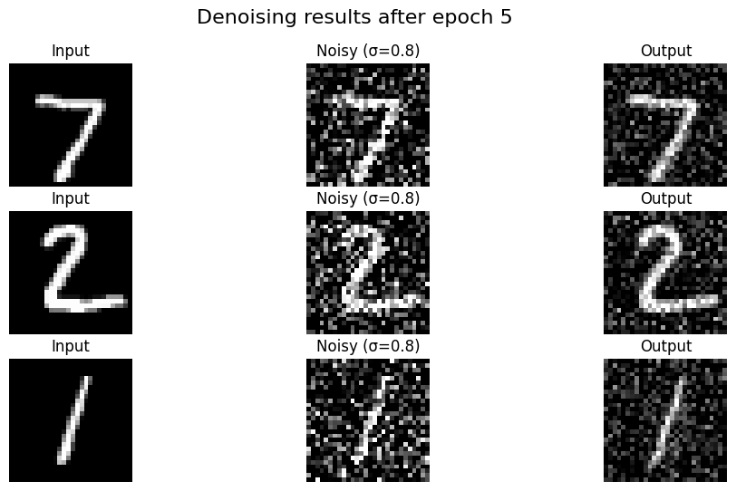$\sigma=0.8$
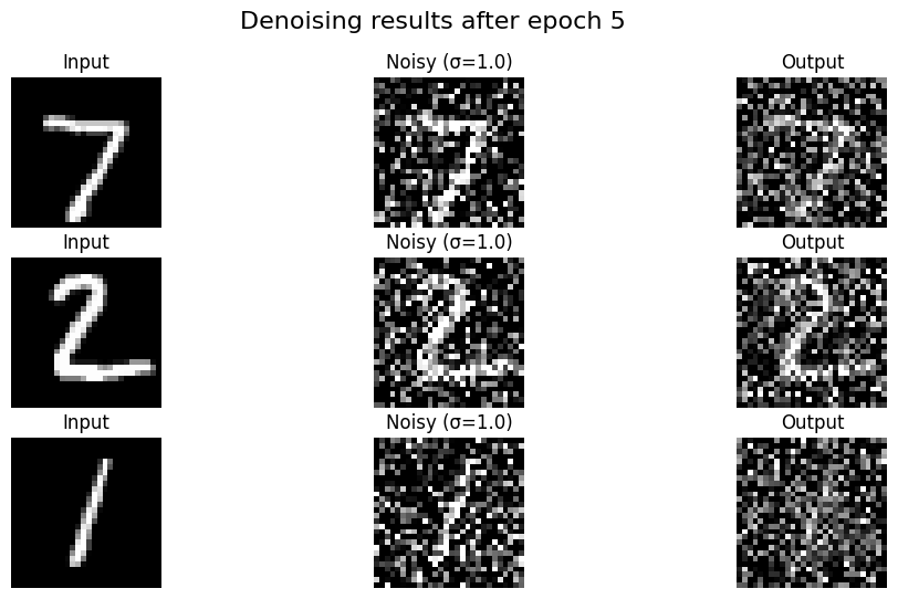$\sigma=1.0$

1.2.3 Denoising Pure Noise

Here, I trained the model to denoise pure noise (i.e., mapping $\mathcal{N}(0, I)$ to MNIST digits).

Interestingly, the model manages to generate digit-like shapes, but they are often blurry or hybrids of multiple digits. This is because the mapping from pure noise to a specific digit is one-to-many and highly ambiguous, so the L2 loss forces the model to output the “average” of all possible digits, resulting in blurry blobs.

2. Training a Diffusion Model

Now we move to a proper diffusion model (Time-Conditioned UNet), where we iteratively denoise the image.

2.1 Adding Time Conditioning

To perform iterative denoising, the model needs to know the current noise level (or timestep $t$). We inject this information into the UNet using fully connected blocks (FCBlocks).

The scalar $t$ is fed into two fully connected blocks (fc1_t, fc2_t) to produce scaling coefficients. These coefficients are then used to modulate the feature maps at specific points in the UNet.

Specifically, $t$ is used to scale the activations after the unflatten step ($t_1$) and after the first upsampling block ($t_2$):

# fc1_t and fc2_t are small MLPs that project the scalar t to channel dimensions
t1 = fc1_t(t)
t2 = fc2_t(t)

# Modulate the unflattened features
unflatten = unflatten * t1

# ... intermediate layers ...

# Modulate the first upsampling block
up1 = up1 * t2

Training involves picking a random image $x_1$, a random timestep $t$, adding noise to get $x_t$, and training the network. The loss at every time step is calculated based on how well the model prediction conditioned on noisy image $x_t$ and time step $t$ matches $x_1 - x_0$: the clean image minus the random noise.

2.2 Time-Conditioned UNet Training

I trained the UNet conditioned on the timestep $t$.

2.3 Time-Conditioned Sampling

Sampling starts from pure noise $x_0 \sim \mathcal{N}(0, 1)$ and iteratively refines it to a clean image $x_1$.

Here are the sampling results at different epochs and different seeds (100, 101, and 102):

2.4 Adding Class-Conditioning to UNet

To improve the generation quality and gain control over the output, we condition the UNet on both the timestep $t$ and the digit class $c$. This allows us to ask the model for a “5” or a “7” specifically.

Architectural Changes

Similar to time conditioning, we inject the class information $c$ (a one-hot vector) into the network. We add two more FCBlocks (fc1_c, fc2_c) to process the class vector.

The class conditioning is added to the time conditioning, meaning the modulation signal becomes a combination of both:

# c is a one-hot vector for the digit class
c1 = fc1_c(c)
c2 = fc2_c(c)

# Combine with time embedding and modulate
unflatten = (c1 * unflatten) + t1
# ...
up1 = (c2 * up1) + t2

We also use dropout on the class conditioning (setting it to a null token with $p=0.1$) to enable Classifier-Free Guidance later.

2.5 Training the UNet

We train the class-conditioned UNet using the same process as before, but with the added class labels.

2.6 Sampling from the UNet

We use Classifier-Free Guidance (CFG) during sampling to improve quality. The final noise estimate is a combination of the conditional and unconditional estimates: \(\epsilon = \epsilon_{uncond} + \gamma (\epsilon_{cond} - \epsilon_{uncond})\)

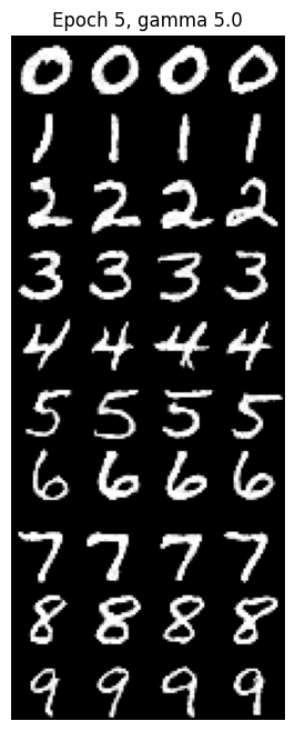
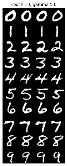
By guiding the model with class labels, we can generate specific digits. Here are the results over 10 epochs using Classifier-Free Guidance ($\gamma=5.0$).

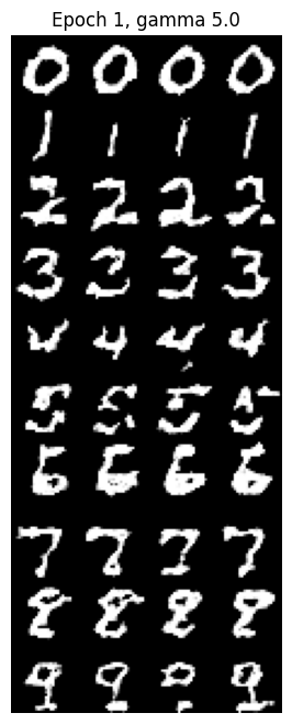
Epoch 1

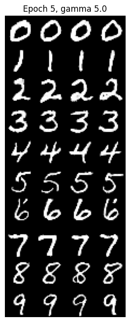
Epoch 5

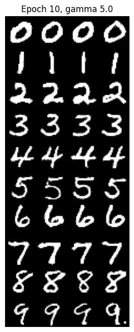
Epoch 10

Can we get rid of the annoying learning rate scheduler?

I tried training the model with a constant learning rate of 1e-4 instead of using an exponential decay scheduler. To account for the fact that the learning rate no longer decreases, I used AdamW with a weight decay of 1e-4. As shown in the loss curve, the training was still stable.

The sampling results are also comparable to the scheduled version, suggesting that for this specific task and architecture, a well-tuned constant learning rate is sufficient.

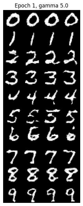
Epoch 1

Epoch 5

Epoch 10