<?xml version="1.0" encoding="utf-8"?><feed xmlns="http://www.w3.org/2005/Atom" ><generator uri="https://jekyllrb.com/" version="3.10.0">Jekyll</generator><link href="https://www.vkethana.com/feed.xml" rel="self" type="application/atom+xml" /><link href="https://www.vkethana.com/" rel="alternate" type="text/html" /><updated>2026-08-10T04:50:21+00:00</updated><id>https://www.vkethana.com/feed.xml</id><title type="html">vkethana.com</title><subtitle>Vijay&apos;s personal website</subtitle><author><name>Vijay Kethanaboyina</name></author><entry><title type="html">Flow Matching Models from Scratch in PyTorch</title><link href="https://www.vkethana.com/diffusion/" rel="alternate" type="text/html" title="Flow Matching Models from Scratch in PyTorch" /><published>2025-12-12T00:00:00+00:00</published><updated>2025-12-12T00:00:00+00:00</updated><id>https://www.vkethana.com/diffusion</id><content type="html" xml:base="https://www.vkethana.com/diffusion/"><![CDATA[<h2 id="table-of-contents">Table of Contents</h2>
<ul>
  <li><a href="#part-0-setup">Part 0: Setup</a></li>
  <li><a href="#part-1-sampling-loops">Part A: Sampling Loops</a>
    <ul>
      <li><a href="#11-implementing-the-forward-process">1.1 Implementing the Forward Process</a></li>
      <li><a href="#12-classical-denoising">1.2 Classical Denoising</a></li>
      <li><a href="#13-one-step-denoising">1.3 One-Step Denoising</a></li>
      <li><a href="#14-iterative-denoising">1.4 Iterative Denoising</a></li>
      <li><a href="#15-diffusion-model-sampling">1.5 Diffusion Model Sampling</a></li>
      <li><a href="#16-classifier-free-guidance-cfg">1.6 Classifier-Free Guidance (CFG)</a></li>
      <li><a href="#17-image-to-image-translation">1.7 Image-to-Image Translation</a></li>
      <li><a href="#18-visual-anagrams">1.8 Visual Anagrams</a></li>
      <li><a href="#19-hybrid-images">1.9 Hybrid Images</a></li>
    </ul>
  </li>
  <li><a href="#part-b-flow-matching-from-scratch">Part B: Flow Matching from Scratch!</a>
    <ul>
      <li><a href="#1-single-step-denoising-unet">1. Single-Step Denoising UNet</a></li>
      <li><a href="#2-training-a-diffusion-model">2. Training a Diffusion Model</a></li>
    </ul>
  </li>
</ul>

<hr />

<h2 id="tldr">TLDR</h2>

<p>In this project, I explore techniques for sampling from pretrained diffusion models <a href="#part-1-sampling-loops">(Part A)</a> and train my own class-conditioned flow matching model from scratch using a UNet <a href="#part-b-flow-matching-from-scratch">(Part B)</a>.</p>


<p>Here’s an example of an image sampled from the model I trained in part B, which can generate images of any handwritten digit between 0 and 9:</p>
<p align="center">
  <img src="/assets/images/diffusion/diffusion.webp" alt="An image being generated from scratch" />
</p>

<h2 id="part-0-setup">Part 0: Setup</h2>

<p>In this part, I experimented with the DeepFloyd IF diffusion model. This is a text-to-image model that operates in two stages:</p>
<ol>
  <li><strong>Stage 1</strong>: Generates a 64x64 resolution image from the text prompt.</li>
  <li><strong>Stage 2</strong>: Upscales the image to 256x256 and adds details.</li>
</ol>

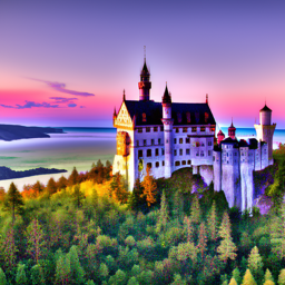
<p>I generated images for three different prompts using 20 inference steps. The random seed used for <em>all parts</em> of this project is <strong>100</strong>.</p>

<h3 id="an-oil-painting-of-a-snowy-mountain-village">“An oil painting of a snowy mountain village”</h3>
<p align="center">
  <img src="/assets/images/diffusion/part0_stage1_castle_20_inference_steps.png" width="200" title="Stage 1" />
  <img src="/assets/images/diffusion/part0_stage2_castle_20_inference_steps.png" width="400" title="Stage 2" />
</p>

<h3 id="a-photo-of-a-cat">“A photo of a cat”</h3>
<p align="center">
  <img src="/assets/images/diffusion/part0_stage1_cat_20_inference_steps.png" width="200" title="Stage 1" />
  <img src="/assets/images/diffusion/part0_stage2_cat_20_inference_steps.png" width="400" title="Stage 2" />
</p>

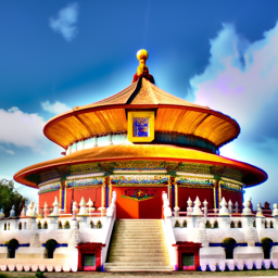
<h3 id="a-photo-of-a-temple">“A photo of a temple”</h3>
<p align="center">
  <img src="/assets/images/diffusion/part0_stage1_temple_20_inference_steps.png" width="200" title="Stage 1 (20 steps)" />
  <img src="/assets/images/diffusion/part0_stage2_temple_20_inference_steps.png" width="400" title="Stage 2 (20 steps)" />
</p>

<p>The outputs here are pretty good in my opinion, which is a testament to the quality of Deepfloyd IF’s training process.</p>

<h4 id="comparison-with-more-inference-steps">Comparison with More Inference Steps</h4>
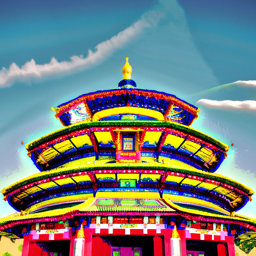
<p>I also generated the temple image with 100 inference steps. This lets us see if the quality improves with more denoising iterations.</p>
<p align="center">
  <img src="/assets/images/diffusion/part0_stage1_temple_100_inference_steps.png" width="200" title="Stage 1 (100 steps)" />
  <img src="/assets/images/diffusion/part0_stage2_temple_100_inference_steps.png" width="400" title="Stage 2 (100 steps)" />
</p>

<p>The image turned out a little bit oversaturated, which makes me believe that more inference steps were not necessary, at least for this specific prompt. 
That said, it didn’t ruin the image either, so my conclusion is that the number of inference steps has to be chosen qualitatively and depends on the prompt and model being used.</p>

<hr />

<h2 id="part-1-sampling-loops">Part 1: Sampling Loops</h2>

<h3 id="11-implementing-the-forward-process">1.1 Implementing the Forward Process</h3>

<p>The forward process in diffusion models adds noise to a clean image $x_0$ to produce a noisy image $x_t$ at timestep $t$. The process is defined by the equation:</p>

\[q(x_t | x_0) = \mathcal{N}(x_t ; \sqrt{\bar\alpha_t} x_0, (1 - \bar\alpha_t)\mathbf{I})\]

<p>Which allows us to sample $x_t$ directly:</p>

\[x_t = \sqrt{\bar\alpha_t} x_0 + \sqrt{1 - \bar\alpha_t} \epsilon, \quad \epsilon \sim \mathcal{N}(0, \mathbf{I})\]

<p>Here are the results of the forward process on the Campanile image at different noise levels ($t \in {250, 500, 750}$):</p>

<p align="center">
  <figure style="display:inline-block; margin:5px;">
    <img src="/assets/images/diffusion/campanile.png" width="150" />
    <figcaption>Original</figcaption>
  </figure>
  <figure style="display:inline-block; margin:5px;">
    <img src="/assets/images/diffusion/part1_1_campanile_250.png" width="150" />
    <figcaption>t=250</figcaption>
  </figure>
  <figure style="display:inline-block; margin:5px;">
    <img src="/assets/images/diffusion/part1_1_campanile_500.png" width="150" />
    <figcaption>t=500</figcaption>
  </figure>
  <figure style="display:inline-block; margin:5px;">
    <img src="/assets/images/diffusion/part1_1_campanile_750.png" width="150" />
    <figcaption>t=750</figcaption>
  </figure>
</p>

<h3 id="12-classical-denoising">1.2 Classical Denoising</h3>

<p>I first attempted to remove the noise using classical Gaussian blurring. As expected, this simple technique fails to recover the details, blurring out both the noise and the high-frequency content of the image.</p>

<p align="center">
  <figure style="display:inline-block; margin:5px;">
    <img src="/assets/images/diffusion/part1_2_campanile_250_blurred.png" width="150" />
    <figcaption>t=250 Blurred</figcaption>
  </figure>
  <figure style="display:inline-block; margin:5px;">
    <img src="/assets/images/diffusion/part1_2_campanile_500_blurred.png" width="150" />
    <figcaption>t=500 Blurred</figcaption>
  </figure>
  <figure style="display:inline-block; margin:5px;">
    <img src="/assets/images/diffusion/part1_2_campanile_750_blurred.png" width="150" />
    <figcaption>t=750 Blurred</figcaption>
  </figure>
</p>

<p>No amount of Gaussian blurring can bring back parts of the image that were already lost. We need something more sophisticated.</p>

<h3 id="13-one-step-denoising">1.3 One-Step Denoising</h3>

<p>Using a pretrained diffusion model, we can try to recover $x_0$ in a single step. The model is trained to estimate the noise $\epsilon$ in a noisy image $x_t$. Given the estimate $\epsilon_\theta(x_t, t)$, we can approximate $x_0$ by inverting the forward process equation:</p>

\[\hat{x}_0 = \frac{x_t - \sqrt{1 - \bar\alpha_t} \epsilon_\theta(x_t, t)}{\sqrt{\bar\alpha_t}}\]

<p align="center">
  <figure style="display:inline-block; margin:5px;">
    <img src="/assets/images/diffusion/part1_3_denoise_250.png" width="150" />
    <figcaption>Denoised (t=250)</figcaption>
  </figure>
  <figure style="display:inline-block; margin:5px;">
    <img src="/assets/images/diffusion/part1_3_denoise_500.png" width="150" />
    <figcaption>Denoised (t=500)</figcaption>
  </figure>
  <figure style="display:inline-block; margin:5px;">
    <img src="/assets/images/diffusion/part1_3_denoise_750.png" width="150" />
    <figcaption>Denoised (t=750)</figcaption>
  </figure>
</p>

<p>The model does a much better job than Gaussian blur, but for high noise levels (t=750), the one-step reconstruction is blurry and lacks fine detail. This is because the initial assumption of mapping directly to $x_0$ is difficult when the signal is heavily corrupted.</p>

<h3 id="14-iterative-denoising">1.4 Iterative Denoising</h3>

<p>To get high-quality images, we denoise iteratively. Starting from pure noise or a noisy image, we repeatedly apply the update step:</p>

\[x_{t'} = \frac{\sqrt{\bar\alpha_{t'}}\beta_t}{1 - \bar\alpha_t} x_0 + \frac{\sqrt{\alpha_t}(1 - \bar\alpha_{t'})}{1 - \bar\alpha_t} x_t + v_\sigma\]

<p>which effectively steps from $t$ to $t’$ by removing a fraction of the predicted noise and adding new variance. In practice, we don’t iteratively denoise over all 1000 timesteps, as that would be too costly. Instead, we iterate over a strided subset of timesteps (for this assignment, I set the stride to 30)</p>

<p>Here is the progression of iterative denoising (using strided sampling):</p>

<p align="center">
  <figure style="display:inline-block; margin:5px;">
    <img src="/assets/images/diffusion/part1_3_step_690_denoise.png" width="120" title="t=690" />
    <figcaption>t=690</figcaption>
  </figure>
  <figure style="display:inline-block; margin:5px;">
    <img src="/assets/images/diffusion/part1_3_step_540_denoise.png" width="120" title="t=540" />
    <figcaption>t=540</figcaption>
  </figure>
  <figure style="display:inline-block; margin:5px;">
    <img src="/assets/images/diffusion/part1_3_step_390_denoise.png" width="120" title="t=390" />
    <figcaption>t=390</figcaption>
  </figure>
  <figure style="display:inline-block; margin:5px;">
    <img src="/assets/images/diffusion/part1_3_step_240_denoise.png" width="120" title="t=240" />
    <figcaption>t=240</figcaption>
  </figure>
  <figure style="display:inline-block; margin:5px;">
    <img src="/assets/images/diffusion/part1_3_step_90_denoise.png" width="120" title="t=90" />
    <figcaption>t=90</figcaption>
  </figure>
</p>

<p><strong>Comparison:</strong></p>
<p align="center">
  <figure style="display:inline-block; margin:5px;">
    <img src="/assets/images/diffusion/part1_3_gaussian_blurred.png" width="150" />
    <figcaption>Gaussian Blur</figcaption>
  </figure>
  <figure style="display:inline-block; margin:5px;">
    <img src="/assets/images/diffusion/part1_3_step_non_iterative_denoise.png" width="150" />
    <figcaption>One-Step</figcaption>
  </figure>
  <figure style="display:inline-block; margin:5px;">
    <img src="/assets/images/diffusion/part1_3_step_final_denoise.png" width="150" />
    <figcaption>Iterative</figcaption>
  </figure>
</p>

<p>The iterative result is significantly sharper than the one-step estimation.</p>

<h3 id="15-diffusion-model-sampling">1.5 Diffusion Model Sampling</h3>

<p>We can generate new images by running the iterative denoising loop starting from pure Gaussian noise ($x_T \sim \mathcal{N}(0, \mathbf{I})$) with the prompt “a high quality photo”.</p>

<p align="center">
  <figure style="display:inline-block; margin:5px;">
    <img src="/assets/images/diffusion/part1_5_sample1.png" width="128" />
  </figure>
  <figure style="display:inline-block; margin:5px;">
    <img src="/assets/images/diffusion/part1_5_sample2.png" width="128" />
  </figure>
  <figure style="display:inline-block; margin:5px;">
    <img src="/assets/images/diffusion/part1_5_sample3.png" width="128" />
  </figure>
  <figure style="display:inline-block; margin:5px;">
    <img src="/assets/images/diffusion/part1_5_sample4.png" width="128" />
  </figure>
  <figure style="display:inline-block; margin:5px;">
    <img src="/assets/images/diffusion/part1_5_sample5.png" width="128" />
  </figure>
</p>

<h3 id="16-classifier-free-guidance-cfg">1.6 Classifier-Free Guidance (CFG)</h3>

<p>To improve image quality and prompt adherence, I implemented Classifier-Free Guidance, also known as CFG. We compute two noise estimates: one conditional on the text prompt ($\epsilon_{cond}$) and one unconditional ($\epsilon_{uncond}$). The final noise estimate is:</p>

\[\epsilon = \epsilon_{uncond} + \gamma (\epsilon_{cond} - \epsilon_{uncond})\]

<p>where $\gamma &gt; 1$ is the guidance scale. This pushes the image towards the prompt.</p>

<p align="center">
  <figure style="display:inline-block; margin:5px;">
    <img src="/assets/images/diffusion/part1_6_sample1.png" width="128" />
  </figure>
  <figure style="display:inline-block; margin:5px;">
    <img src="/assets/images/diffusion/part1_6_sample2.png" width="128" />
  </figure>
  <figure style="display:inline-block; margin:5px;">
    <img src="/assets/images/diffusion/part1_6_sample3.png" width="128" />
  </figure>
  <figure style="display:inline-block; margin:5px;">
    <img src="/assets/images/diffusion/part1_6_sample4.png" width="128" />
  </figure>
  <figure style="display:inline-block; margin:5px;">
    <img src="/assets/images/diffusion/part1_6_sample5.png" width="128" />
  </figure>
</p>

<p>The generated images are sharper and more clearly defined compared to the unguided samples.</p>

<h3 id="17-image-to-image-translation">1.7 Image-to-Image Translation</h3>
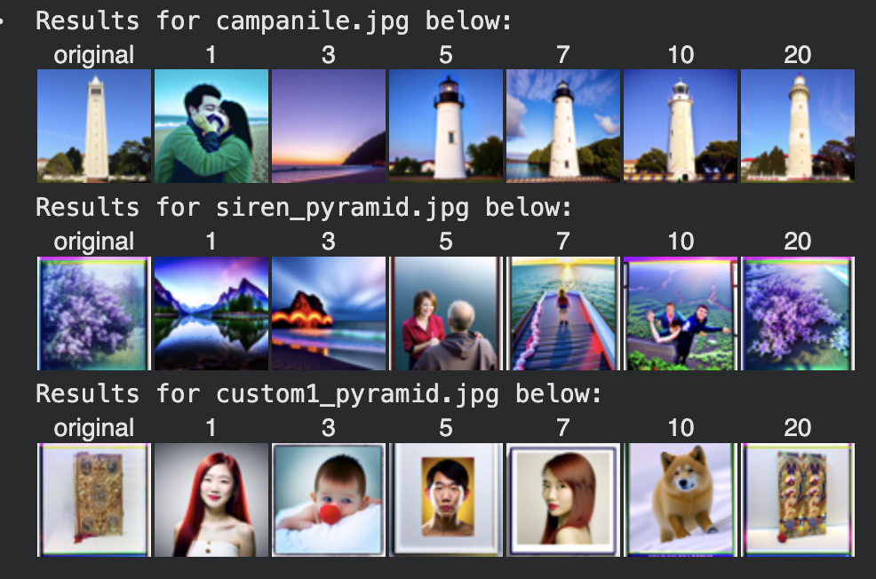
<p>By taking a real image, adding noise to it up to a certain timestep $t$, and then running the iterative denoising process from there, we can edit images. This allows us to balance maintaining the original structure (via the starting noisy image) and generating new details (via the denoising loop).</p>

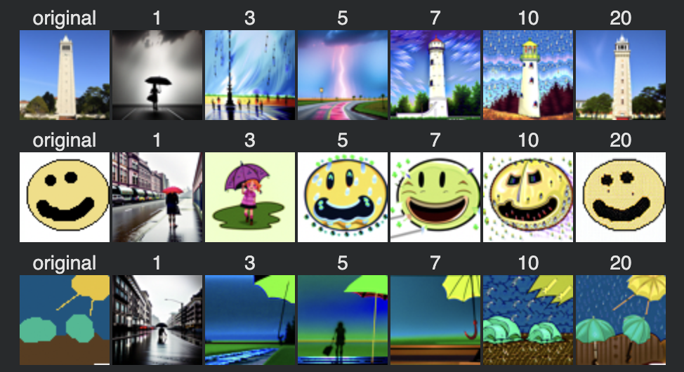
<p>Below I show edits of the Campanile image at noise levels [1, 3, 5, 7, 10, 20] with the conditional text prompt “a high quality photo”.
I also show two edits of my own test images, which are captioned “original” in the below image:</p>

<p align="center">
  <img src="/assets/images/diffusion/part1_7_im2_im.png" width="512" title="Original/Mask" />
</p>
<h4 id="171-sdedit">1.7.1 SDEdit</h4>

<p><strong>Artificial Image Transition (SDEdit):</strong></p>
<p align="center">
  <img src="/assets/images/diffusion/part1_7_1_artificial_img.png" width="150" title="Original" />
  <img src="/assets/images/diffusion/part1_7_1_artificial_img_transition.png" width="500" title="Transition" />
</p>

<p><strong>Hand-Drawn Image Transition:</strong></p>
<p align="center">
  <img src="/assets/images/diffusion/part1_7_1_drawn1.png" width="150" title="Sketch 1" />
  <img src="/assets/images/diffusion/part1_7_1_drawn1_transition.png" width="500" title="Transition 1" />
</p>
<p align="center">
  <img src="/assets/images/diffusion/part1_7_1_drawn2.png" width="150" title="Sketch 2" />
  <img src="/assets/images/diffusion/part1_7_1_drawn2_transition.png" width="500" title="Transition 2" />
</p>

<h4 id="172-inpainting">1.7.2 Inpainting</h4>
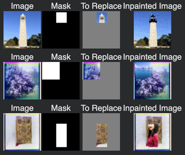
<p>We can use a mask to keep parts of the image constant while denoising the rest. At each step of the backward process, we force the pixels outside the mask to match the noisy version of the original image, while letting the model hallucinate content inside the mask.</p>

<p align="center">
  <img src="/assets/images/diffusion/part1_7_2.png" width="512" title="Inpainted Result" />
</p>

<h4 id="173-text-conditional-image-to-image-translation">1.7.3 Text-Conditional Image-to-Image Translation</h4>
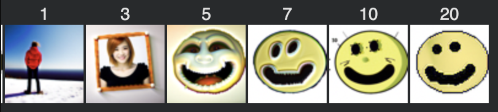
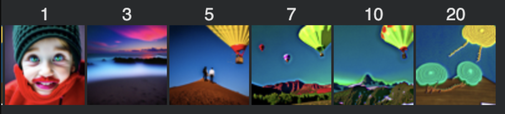
<p>We can guide the SDEdit process with specific text prompts to change the style or content of the image.
Results for all three images are below:</p>

<p>Here, the prompt was “a rainy day”. Notice now the images gradually have more and more “rain-like” features. For example, the campanile turns into a bolt of lightning for time step 5 of the first row. Similarly, the happy face drawing starts to show small droplets of rain on its sides.</p>

<p align="center">
  <img src="/assets/images/diffusion/part_1_7_3.png" width="512" title="Text-Guided Edit" />
</p>

<h3 id="18-visual-anagrams">1.8 Visual Anagrams</h3>

<p>Visual anagrams are images that look like one thing when upright and another when flipped. I implemented this by averaging the noise estimates for two different prompts, one computed on the upright image and one on the flipped image:</p>

\[\epsilon_{final} = \frac{1}{2} (\epsilon_\theta(x_t, t, p_1) + \text{flip}(\epsilon_\theta(\text{flip}(x_t), t, p_2)))\]

<p align="center">
  <figure style="display:inline-block; margin:5px;">
    <img src="/assets/images/diffusion/part1_8_castle_skull.png" width="200" />
    <figcaption>Upright: Castle/Village</figcaption>
  </figure>
  <figure style="display:inline-block; margin:5px;">
    <img src="/assets/images/diffusion/part1_8_castle_skull_flipped.png" width="200" />
    <figcaption>Flipped: Skull</figcaption>
  </figure>
</p>

<p align="center">
  <figure style="display:inline-block; margin:5px;">
    <img src="/assets/images/diffusion/part1_8_citadel_castle.png" width="200" />
    <figcaption>Upright: Citadel</figcaption>
  </figure>
  <figure style="display:inline-block; margin:5px;">
    <img src="/assets/images/diffusion/part1_8_citadel_castle_flipped.png" width="200" />
    <figcaption>Flipped: Temple</figcaption>
  </figure>
</p>

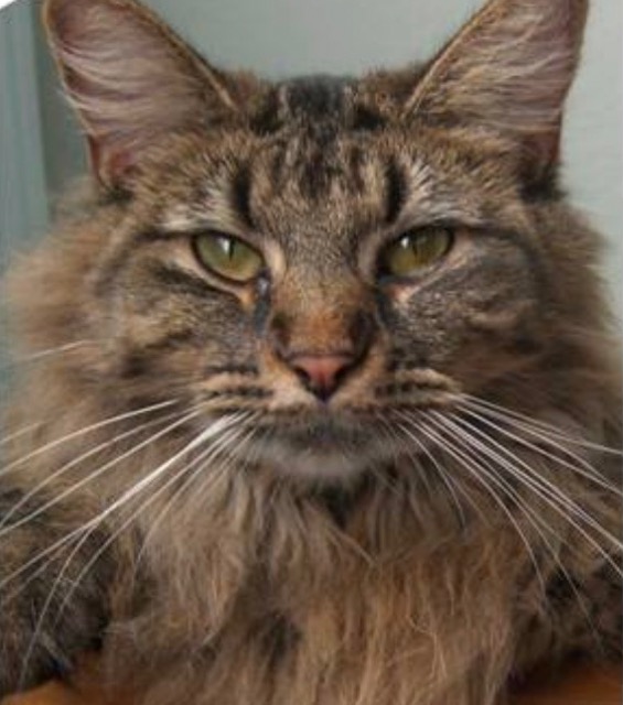
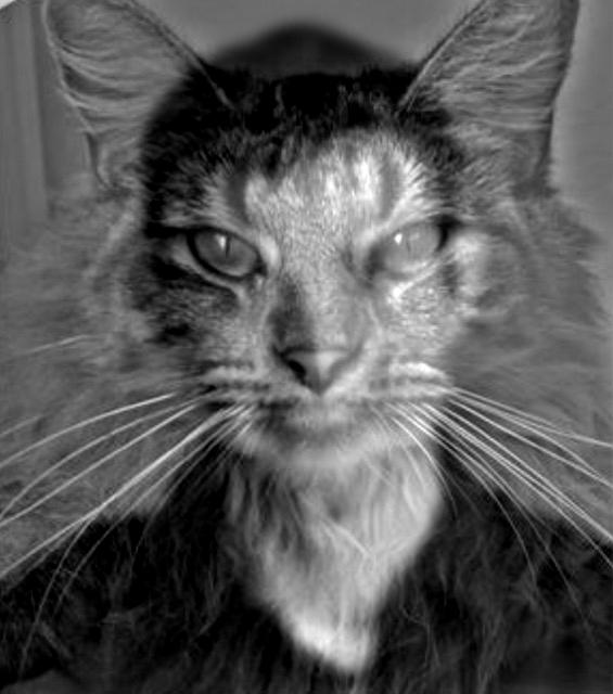
<h3 id="19-hybrid-images">1.9 Hybrid Images</h3>

<p>Hybrid images combine the low frequencies of one image with the high frequencies of another. We can generate these with diffusion by combining noise estimates:</p>

\[\epsilon_{final} = f_{low}(\epsilon_\theta(x_t, t, p_1)) + f_{high}(\epsilon_\theta(x_t, t, p_2))\]

<p align="center">
  <figure style="display:inline-block; margin:5px;">
    <img src="/assets/images/diffusion/part1_9_hybrid1.png" width="200" />
    <figcaption>Hybrid Image 1: Rainy Day + Photo of Dog</figcaption>
  </figure>
  <figure style="display:inline-block; margin:5px;">
    <img src="/assets/images/diffusion/part1_9_hybrid2.png" width="200" />
    <figcaption>Hybrid Image 2: A lithograph of a skull + photo of a castle</figcaption>
  </figure>
</p>

<hr />

<h1 id="part-b-flow-matching-from-scratch">Part B: Flow Matching from Scratch!</h1>

<p>In this part, we implement a diffusion model from scratch using the MNIST dataset. We start with a simple single-step denoiser and then move on to a full diffusion model with time conditioning. Unless otherwise stated, the random seed used for all subparts was <strong>100</strong>.</p>

<h2 id="1-single-step-denoising-unet">1. Single-Step Denoising UNet</h2>

<h3 id="11-architecture">1.1 Architecture</h3>
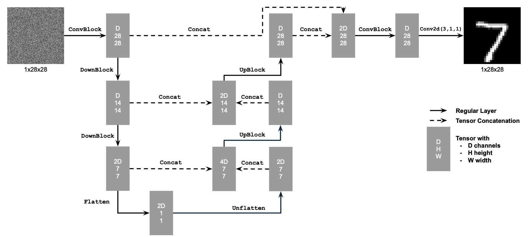
<p>The backbone of our denoiser is a UNet. At its core, a UNet is just an autoencoder with a twist: it compresses the image into a bottleneck to capture global context (like “this is a digit 8”) and then expands it back to the original size. The “twist” is the skip connections—wires that bypass the bottleneck and plug the detailed, high-resolution features from the encoder directly into the decoder. This lets the network reconstruct fine details (like edges and noise) that would otherwise be lost in compression.</p>

<p align="center">
  <img src="/assets/images/diffusion/part2/unconditional_arch.png" width="700" title="UNet Architecture" />
</p>

<h3 id="12-noising-process-visualization">1.2 Noising Process Visualization</h3>
<p>The noising process adds Gaussian noise to a clean image $x$.
\(z = x + \sigma \epsilon, \quad \epsilon \sim \mathcal{N}(0, I)\)</p>

<p>Here is the effect of varying $\sigma$ on a clean image:</p>

<p align="center">
  <img src="/assets/images/diffusion/part2/part_1_2_noising_process.png" width="661" title="Noising Process" />
</p>

<h3 id="121-training-the-denoiser">1.2.1 Training the Denoiser</h3>
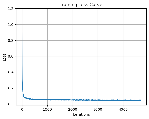
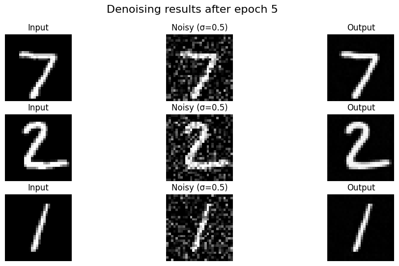
<p>I trained a UNet to denoise images with $\sigma = 0.5$. The objective is to minimize the L2 distance between the denoised image and the original clean image:
\(L = \mathbb{E}_{z,x} \|D_{\theta}(z) - x\|^2\)</p>

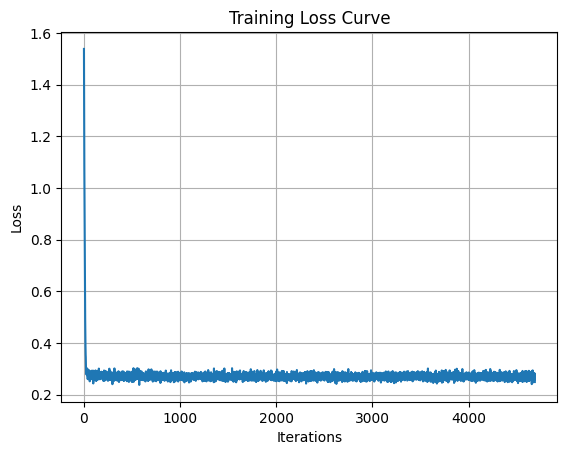
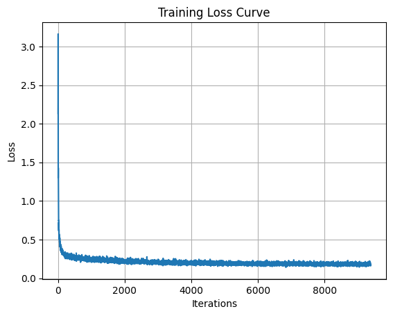
<p><strong>Training Loss Curve:</strong></p>
<p align="center">
  <img src="/assets/images/diffusion/part2/part_1_2_1_plot.png" width="567" title="Training Loss" />
</p>

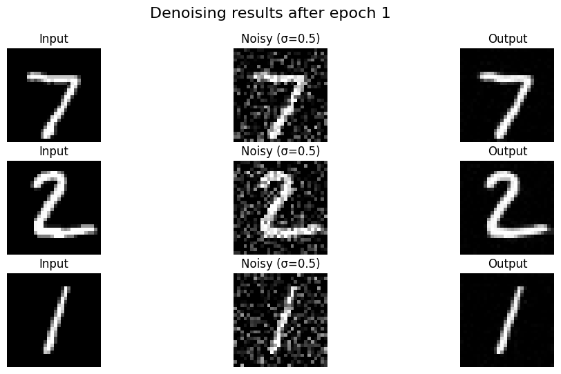
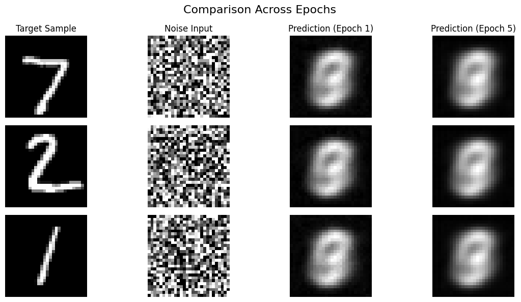
<p><strong>Denoising Results (Epoch 1 vs Epoch 5):</strong>
The model learns to remove the noise effectively after just a few epochs.</p>
<p align="center">
  <figure style="display:block; margin:40px auto;">
    <img src="/assets/images/diffusion/part2/part_1_2_epoch1_denoise_results.png" width="800" />
    <figcaption>Epoch 1</figcaption>
  </figure>
  <figure style="display:block; margin:40px auto;">
    <img src="/assets/images/diffusion/part2/part_1_2_epoch5_denoise_results.png" width="800" />
    <figcaption>Epoch 5</figcaption>
  </figure>
</p>

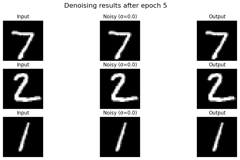
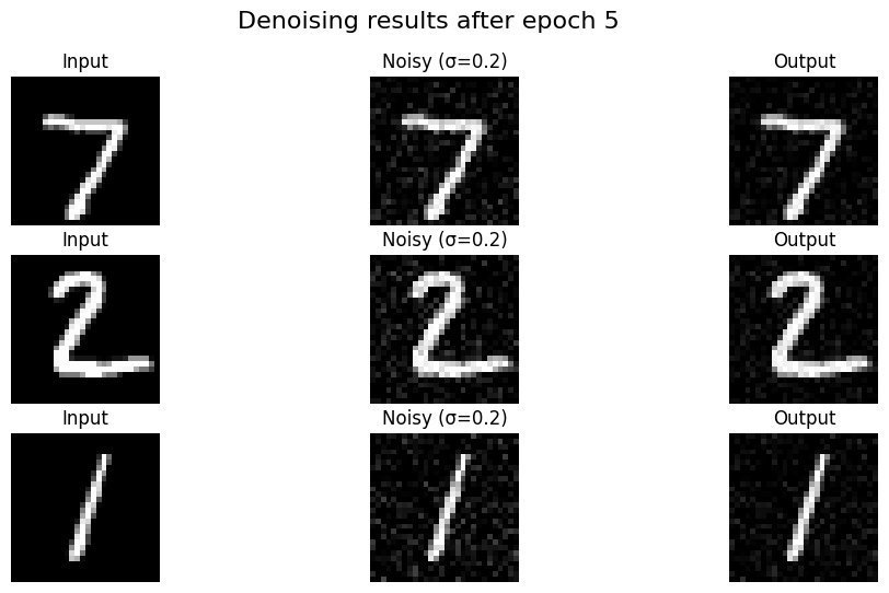
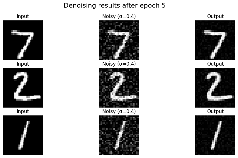
<h3 id="122-out-of-distribution-testing">1.2.2 Out-of-Distribution Testing</h3>
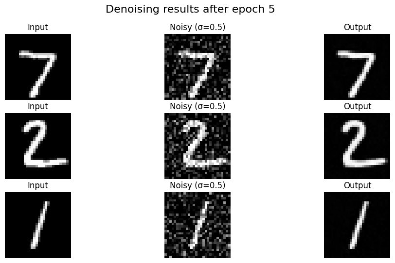
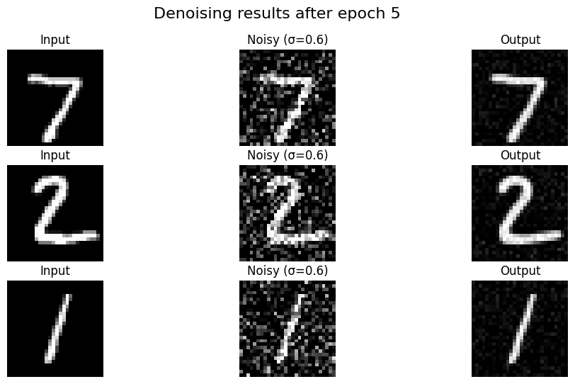
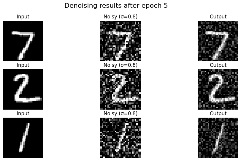
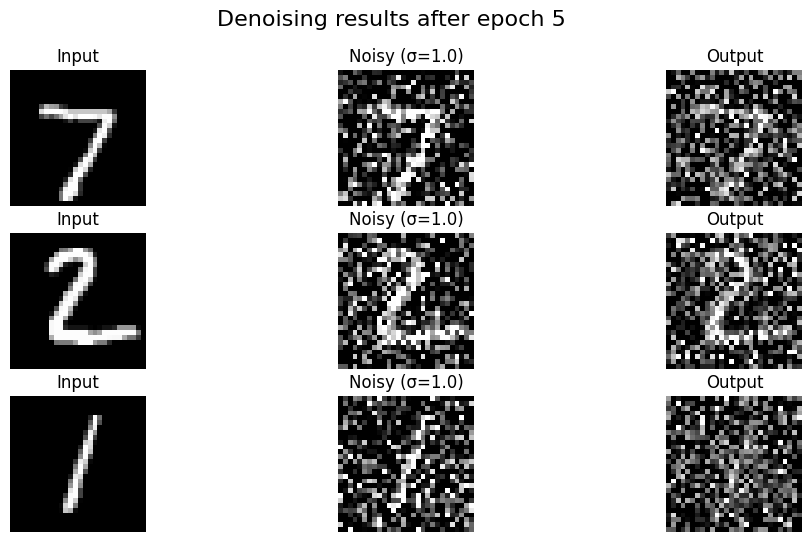
<p>The model was trained only on $\sigma=0.5$. Here I tested it on other noise levels. It performs reasonably well on lower noise levels but struggles when the noise level is much higher than what it was trained on (e.g., $\sigma=1.0$).</p>

<div align="center">
  <table>
    <tr>
      <td align="center">
        <img src="/assets/images/diffusion/part2/part_1_2_ood_sigma_0.png" width="300" />
        $\sigma=0.0$
      </td>
      <td align="center">
        <img src="/assets/images/diffusion/part2/part_1_2_ood_sigma_0.2.png" width="300" />
        $\sigma=0.2$
      </td>
    </tr>
    <tr>
      <td align="center">
        <img src="/assets/images/diffusion/part2/part_1_2_ood_sigma_0.4.png" width="300" />
        $\sigma=0.4$
      </td>
      <td align="center">
        <img src="/assets/images/diffusion/part2/part_1_2_ood_sigma_0.5.png" width="300" />
        $\sigma=0.5$
      </td>
    </tr>
    <tr>
      <td align="center">
        <img src="/assets/images/diffusion/part2/part_1_2_ood_sigma_0.6.png" width="300" />
        $\sigma=0.6$
      </td>
      <td align="center">
        <img src="/assets/images/diffusion/part2/part_1_2_ood_sigma_0.8.png" width="300" />
        $\sigma=0.8$
      </td>
    </tr>
    <tr>
      <td align="center">
        <img src="/assets/images/diffusion/part2/part_1_2_ood_sigma_1.0.png" width="300" />
        $\sigma=1.0$
      </td>
      <td></td> 
    </tr>
  </table>
</div>

<h3 id="123-denoising-pure-noise">1.2.3 Denoising Pure Noise</h3>
<p>Here, I trained the model to denoise pure noise (i.e., mapping $\mathcal{N}(0, I)$ to MNIST digits).</p>

<p align="center">
  <img src="/assets/images/diffusion/part2/part_1_2_3_pure_noise_loss_curve.png" width="567" title="Loss Curve" />
</p>

<p align="center">
  <img src="/assets/images/diffusion/part2/part_1_2_3_generate_from_pure_noise.png" width="800" title="Results" />
</p>

<p>Interestingly, the model manages to generate digit-like shapes, but they are often blurry or hybrids of multiple digits. 
This is because the mapping from pure noise to a specific digit is one-to-many and highly ambiguous, so the L2 loss forces the model to output the “average” of all possible digits, resulting in blurry blobs.</p>

<hr />

<h2 id="2-training-a-diffusion-model">2. Training a Diffusion Model</h2>

<p>Now we move to a proper diffusion model (Time-Conditioned UNet), where we iteratively denoise the image.</p>

<h3 id="21-adding-time-conditioning">2.1 Adding Time Conditioning</h3>
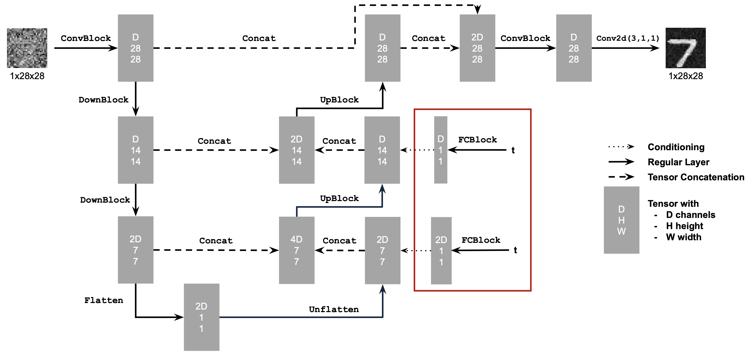
<p>To perform iterative denoising, the model needs to know the current noise level (or timestep $t$). We inject this information into the UNet using fully connected blocks (FCBlocks).</p>

<p align="center">
  <img src="/assets/images/diffusion/part2/conditional_arch_fm.png" width="600" title="Conditioned UNet" />
</p>

<p>The scalar $t$ is fed into two fully connected blocks (<code class="language-plaintext highlighter-rouge">fc1_t</code>, <code class="language-plaintext highlighter-rouge">fc2_t</code>) to produce scaling coefficients. These coefficients are then used to modulate the feature maps at specific points in the UNet.</p>

<p>Specifically, $t$ is used to scale the activations after the unflatten step ($t_1$) and after the first upsampling block ($t_2$):</p>

<div class="language-python highlighter-rouge"><div class="highlight"><pre class="highlight"><code><span class="c1"># fc1_t and fc2_t are small MLPs that project the scalar t to channel dimensions
</span><span class="n">t1</span> <span class="o">=</span> <span class="n">fc1_t</span><span class="p">(</span><span class="n">t</span><span class="p">)</span>
<span class="n">t2</span> <span class="o">=</span> <span class="n">fc2_t</span><span class="p">(</span><span class="n">t</span><span class="p">)</span>

<span class="c1"># Modulate the unflattened features
</span><span class="n">unflatten</span> <span class="o">=</span> <span class="n">unflatten</span> <span class="o">*</span> <span class="n">t1</span>

<span class="c1"># ... intermediate layers ...
</span>
<span class="c1"># Modulate the first upsampling block
</span><span class="n">up1</span> <span class="o">=</span> <span class="n">up1</span> <span class="o">*</span> <span class="n">t2</span>
</code></pre></div></div>

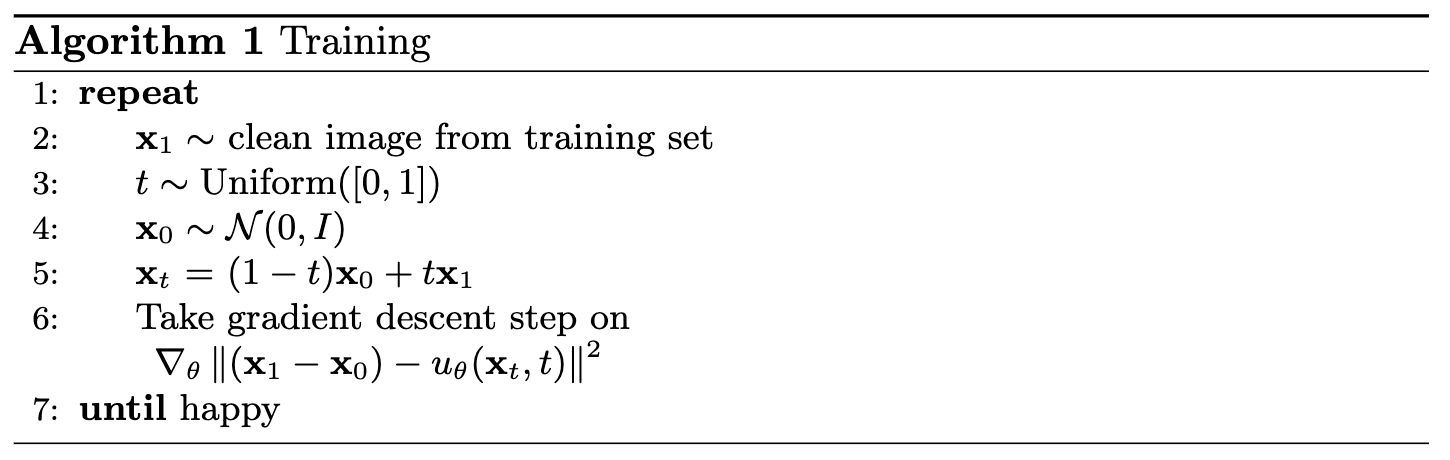
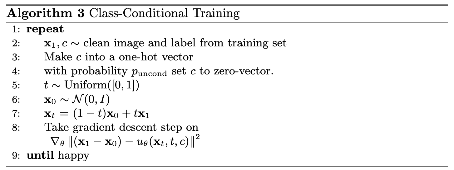
<p>Training involves picking a random image $x_1$, a random timestep $t$, adding noise to get $x_t$, and training the network.
The loss at every time step is calculated based on how well the model prediction conditioned on noisy image $x_t$ and time step $t$ matches $x_1 - x_0$: the clean image <em>minus</em> the random noise.</p>

<p align="center">
  <img src="/assets/images/diffusion/part2/algo1_t_only_fm.png" width="600" title="Training Algorithm" />
</p>

<h3 id="22-time-conditioned-unet-training">2.2 Time-Conditioned UNet Training</h3>
<p>I trained the UNet conditioned on the timestep $t$.</p>

<p align="center">
  <img src="/assets/images/diffusion/part2/part2_2_time_conditioned_unet_plot.png" width="567" title="Time-Conditioned Loss" />
</p>

<h3 id="23-time-conditioned-sampling">2.3 Time-Conditioned Sampling</h3>
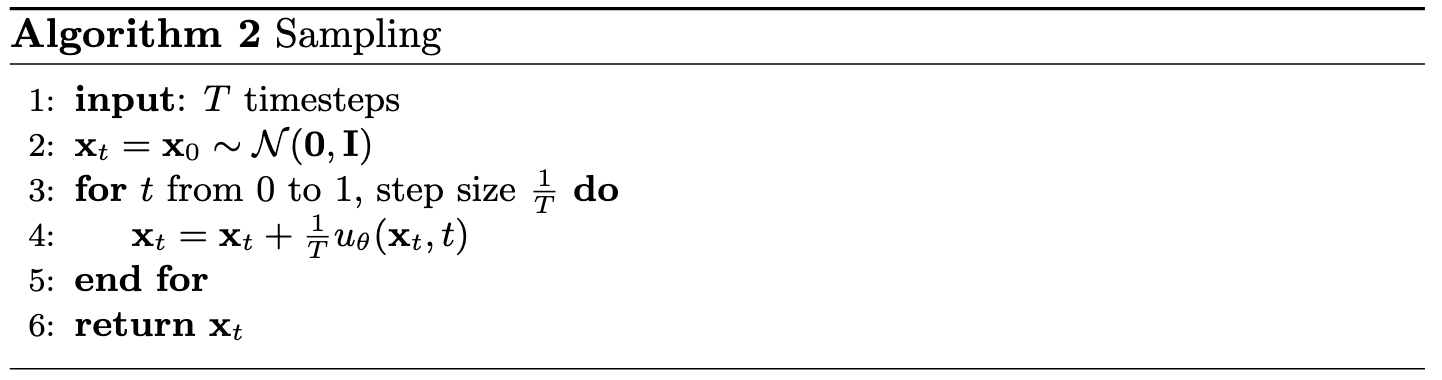
<p>Sampling starts from pure noise $x_0 \sim \mathcal{N}(0, 1)$ and iteratively refines it to a clean image $x_1$.</p>

<p align="center">
  <img src="/assets/images/diffusion/part2/algo2_t_only_fm.png" width="800" title="Sampling Algorithm" />
</p>

<p>Here are the sampling results at different epochs and different seeds (100, 101, and 102):</p>

<p align="center">
  <img src="/assets/images/diffusion/part2/part2_3.png" width="717" title="Sampling Results" />
</p>

<p align="center">
  <img src="/assets/images/diffusion/part2/part2_3_ex2.png" width="717" title="Sampling Results" />
</p>

<p align="center">
  <img src="/assets/images/diffusion/part2/part2_3_ex3.png" width="717" title="Sampling Results" />
</p>

<h3 id="24-adding-class-conditioning-to-unet">2.4 Adding Class-Conditioning to UNet</h3>

<p>To improve the generation quality and gain control over the output, we condition the UNet on both the timestep $t$ and the digit class $c$. This allows us to ask the model for a “5” or a “7” specifically.</p>

<h4 id="architectural-changes">Architectural Changes</h4>
<p>Similar to time conditioning, we inject the class information $c$ (a one-hot vector) into the network. We add two more FCBlocks (<code class="language-plaintext highlighter-rouge">fc1_c</code>, <code class="language-plaintext highlighter-rouge">fc2_c</code>) to process the class vector.</p>

<p>The class conditioning is added to the time conditioning, meaning the modulation signal becomes a combination of both:</p>

<div class="language-python highlighter-rouge"><div class="highlight"><pre class="highlight"><code><span class="c1"># c is a one-hot vector for the digit class
</span><span class="n">c1</span> <span class="o">=</span> <span class="n">fc1_c</span><span class="p">(</span><span class="n">c</span><span class="p">)</span>
<span class="n">c2</span> <span class="o">=</span> <span class="n">fc2_c</span><span class="p">(</span><span class="n">c</span><span class="p">)</span>

<span class="c1"># Combine with time embedding and modulate
</span><span class="n">unflatten</span> <span class="o">=</span> <span class="p">(</span><span class="n">c1</span> <span class="o">*</span> <span class="n">unflatten</span><span class="p">)</span> <span class="o">+</span> <span class="n">t1</span>
<span class="c1"># ...
</span><span class="n">up1</span> <span class="o">=</span> <span class="p">(</span><span class="n">c2</span> <span class="o">*</span> <span class="n">up1</span><span class="p">)</span> <span class="o">+</span> <span class="n">t2</span>
</code></pre></div></div>

<p>We also use dropout on the class conditioning (setting it to a null token with $p=0.1$) to enable Classifier-Free Guidance later.</p>

<p align="center">
  <img src="/assets/images/diffusion/part2/algo3_c_fm.png" width="600" title="Class-Conditioned Training" />
</p>

<h3 id="25-training-the-unet">2.5 Training the UNet</h3>

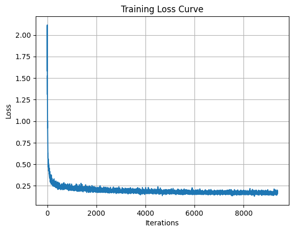
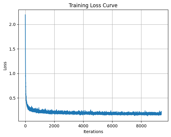
<p>We train the class-conditioned UNet using the same process as before, but with the added class labels.</p>

<p align="center">
  <img src="/assets/images/diffusion/part2/part_2_5_lr_sch_loss_curve.png" width="576" title="Class-Conditioned Loss" />
</p>

<h3 id="26-sampling-from-the-unet">2.6 Sampling from the UNet</h3>

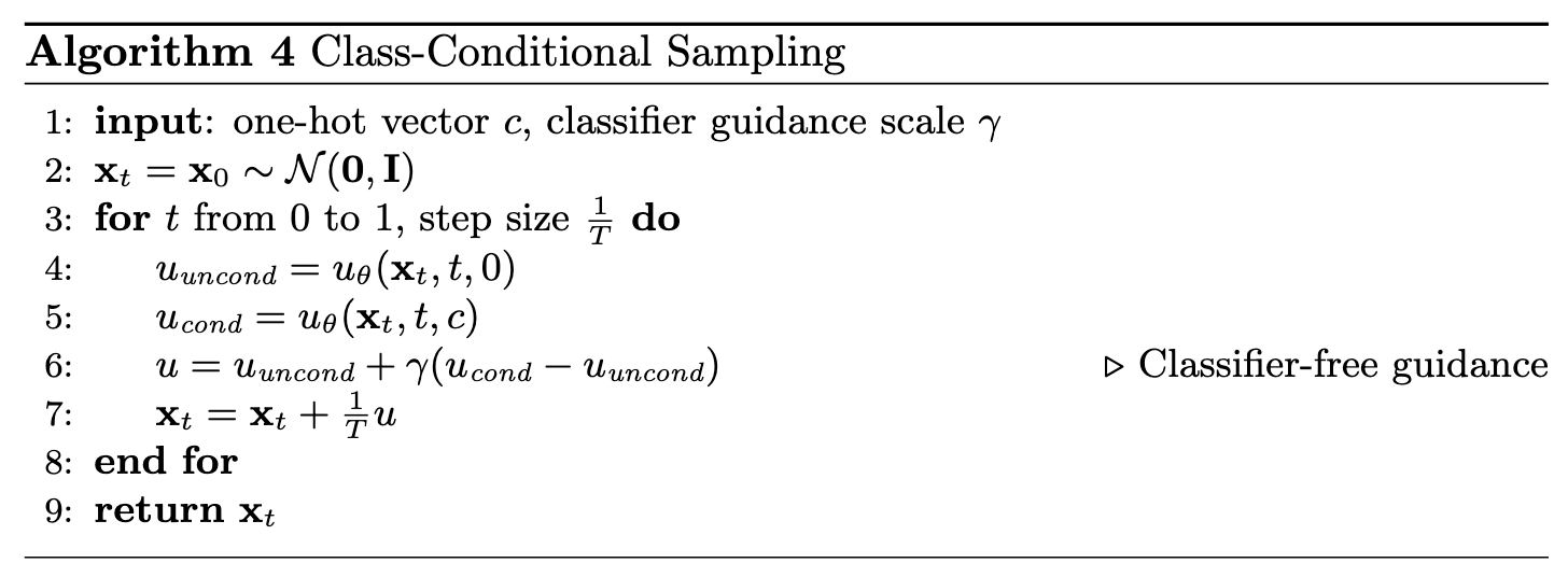
<p>We use Classifier-Free Guidance (CFG) during sampling to improve quality. The final noise estimate is a combination of the conditional and unconditional estimates:
\(\epsilon = \epsilon_{uncond} + \gamma (\epsilon_{cond} - \epsilon_{uncond})\)</p>

<p align="center">
  <img src="/assets/images/diffusion/part2/algo4_c_fm.png" width="600" title="CFG Sampling" />
</p>

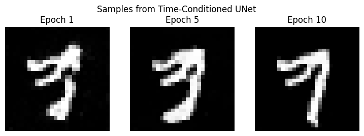
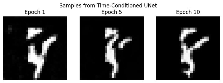
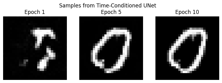
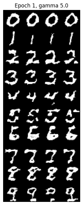
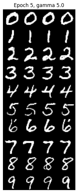
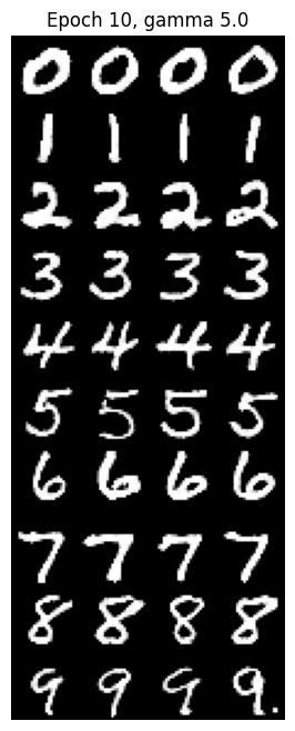
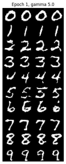
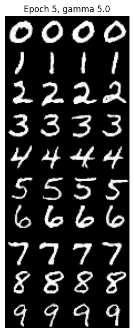
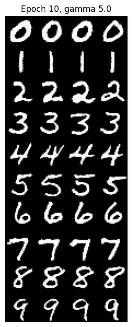
<p>By guiding the model with class labels, we can generate specific digits. Here are the results over 10 epochs using Classifier-Free Guidance ($\gamma=5.0$).</p>

<div align="center">
  <table>
    <tr>
      <td align="center">
        <img src="/assets/images/diffusion/part2/part_2_6_with_lr_sch_epoch1.png" width="220" />
        <br />
        Epoch 1
      </td>
      <td align="center">
        <img src="/assets/images/diffusion/part2/part_2_6_with_lr_sch_epoch5.png" width="220" />
        <br />
        Epoch 5
      </td>
      <td align="center">
        <img src="/assets/images/diffusion/part2/part_2_6_with_lr_sch_epoch10.png" width="220" />
        <br />
        Epoch 10
      </td>
    </tr>
  </table>
</div>

<h4 id="can-we-get-rid-of-the-annoying-learning-rate-scheduler">Can we get rid of the annoying learning rate scheduler?</h4>

<p>I tried training the model with a constant learning rate of 1e-4 instead of using an exponential decay scheduler. To account for the fact that the learning rate no longer decreases, I used AdamW with a weight decay of <strong>1e-4</strong>. As shown in the loss curve, the training was still stable.</p>

<p align="center">
  <img src="/assets/images/diffusion/part2/part_2_5_constant_lr_loss_curve.png" width="567" title="Constant LR Loss" />
</p>

<p>The sampling results are also comparable to the scheduled version, suggesting that for this specific task and architecture, a well-tuned constant learning rate is sufficient.</p>

<div align="center">
  <table>
    <tr>
      <td align="center">
        <img src="/assets/images/diffusion/part2/part_2_6_constant_lr_epoch1.png" width="220" />
        <br />
        Epoch 1
      </td>
      <td align="center">
        <img src="/assets/images/diffusion/part2/part_2_6_constant_lr_epoch5.png" width="220" />
        <br />
        Epoch 5
      </td>
      <td align="center">
        <img src="/assets/images/diffusion/part2/part_2_6_constant_lr_epoch10.png" width="220" />
        <br />
        Epoch 10
      </td>
    </tr>
  </table>
</div>]]></content><author><name>Vijay Kethanaboyina</name></author><category term="machine learning" /><category term="school project" /><summary type="html"><![CDATA[Table of Contents Part 0: Setup Part A: Sampling Loops 1.1 Implementing the Forward Process 1.2 Classical Denoising 1.3 One-Step Denoising 1.4 Iterative Denoising 1.5 Diffusion Model Sampling 1.6 Classifier-Free Guidance (CFG) 1.7 Image-to-Image Translation 1.8 Visual Anagrams 1.9 Hybrid Images Part B: Flow Matching from Scratch! 1. Single-Step Denoising UNet 2. Training a Diffusion Model]]></summary></entry><entry><title type="html">Interactively Visualizing the Qwen3 MoE Architecture</title><link href="https://www.vkethana.com/qwen-arch/" rel="alternate" type="text/html" title="Interactively Visualizing the Qwen3 MoE Architecture" /><published>2025-12-06T00:00:00+00:00</published><updated>2025-12-06T00:00:00+00:00</updated><id>https://www.vkethana.com/qwen-arch</id><content type="html" xml:base="https://www.vkethana.com/qwen-arch/"><![CDATA[<!DOCTYPE html>
<html lang="en">
  <head>
    <meta charset="UTF-8" />
    <meta name="viewport" content="width=device-width, initial-scale=1.0" />
    <title>Interactive Qwen3 (Dense) Diagram</title>
    <style>
      :root {
        color-scheme: light;
        --accent: #1d4ed8;
        --accent-light: #dbeafe;
        --gray: #e2e8f0;
        --tooltip-bg: #1f2937;
      }

      .concepts {
        margin: 48px auto;
        max-width: 760px;
        padding: 0 16px;
        display: grid;
        gap: 18px;
      }

      .concepts h2 {
        margin: 0;
        font-size: 20px;
        color: var(--accent);
      }

      .concept {
        display: grid;
        gap: 6px;
      }

      .concept strong {
        font-size: 16px;
        color: #0f172a;
      }

      .concept p {
        margin: 0;
        font-size: 14px;
        line-height: 1.6;
        color: #334155;
      }

      .page {
        max-width: 900px;
        width: 100%;
        display: flex;
        flex-direction: column;
        align-items: center;
        gap: 24px;
        margin: 24px auto 48px;
        padding: 0 16px;
      }

      .post-intro {
        max-width: 720px;
        margin: 16px auto 32px;
        padding: 0 16px;
        font-size: 1rem;
        line-height: 1.7;
      }

      h1 {
        margin: 0;
        letter-spacing: 0.04em;
        color: var(--accent);
      }

      .tabs {
        display: flex;
        gap: 12px;
        border-bottom: 2px solid var(--accent);
        padding-bottom: 8px;
      }

      .tab {
        padding: 8px 16px;
        border-radius: 10px 10px 0 0;
        background: var(--accent-light);
        border: 2px solid var(--accent);
        border-bottom: none;
        cursor: pointer;
        font-weight: 600;
        color: var(--accent);
        transition: background 0.2s ease;
      }

      .tab.inactive {
        background: #fff;
        color: #1f2937;
        opacity: 0.8;
      }

      .tab-content {
        display: none;
        width: 100%;
        justify-content: center;
      }

      .tab-content.active {
        display: flex;
      }

      .diagram {
        position: relative;
        width: min(680px, 95vw);
        display: flex;
        flex-direction: column;
        align-items: center;
        gap: 16px;
      }

      .component {
        position: relative;
        padding: 12px 18px;
        border: 2px solid var(--accent);
        border-radius: 10px;
        background: white;
        text-align: center;
        font-weight: 600;
        width: clamp(280px, 36vw, 340px);
        box-shadow: 0 2px 6px rgba(15, 23, 42, 0.08);
        transition: transform 0.2s ease;
        z-index: 1;
      }

      .component:hover {
        transform: translateY(-3px);
        z-index: 30;
      }

      .component::after {
        content: attr(data-description);
        position: absolute;
        left: 50%;
        top: 100%;
        transform: translate(-50%, 12px);
        width: clamp(240px, 60vw, 320px);
        background: var(--tooltip-bg);
        color: white;
        padding: 12px;
        border-radius: 8px;
        font-size: 14px;
        line-height: 1.35;
        box-shadow: 0 6px 16px rgba(15, 23, 42, 0.25);
        opacity: 0;
        pointer-events: none;
        transition: opacity 0.15s ease;
        z-index: 10;
      }

      .component:hover::after,
      .adder:hover::after {
        opacity: 1;
      }

      .outer-block {
        width: 100%;
        max-width: 520px;
        background: var(--gray);
        border: 2px solid var(--accent);
        border-radius: 18px;
        padding: 24px 20px 32px;
        display: flex;
        flex-direction: column;
        align-items: center;
        gap: 12px;
        position: relative;
      }

      .inner-block {
        width: 100%;
        background: var(--accent-light);
        border-radius: 14px;
        border: 2px solid var(--accent);
        padding: 20px 20px 24px;
        display: flex;
        flex-direction: column;
        align-items: center;
        gap: 12px;
      }

      .connector {
        width: 6px;
        height: 32px;
        background: var(--accent);
        border-radius: 999px;
      }

      .connector.small {
        height: 24px;
      }

      .adder {
        position: relative;
        width: 36px;
        height: 36px;
        border-radius: 50%;
        border: 2px solid var(--accent);
        background: white;
        display: grid;
        place-items: center;
        font-weight: 700;
        color: var(--accent);
        box-shadow: 0 3px 8px rgba(15, 23, 42, 0.12);
        cursor: help;
        z-index: 1;
        transition: transform 0.2s ease;
      }

      .adder:hover {
        transform: translateY(-2px);
        z-index: 30;
      }

      .adder::after {
        content: attr(data-description);
        position: absolute;
        left: 50%;
        top: 100%;
        transform: translate(-50%, 12px);
        width: 220px;
        background: var(--tooltip-bg);
        color: white;
        padding: 10px;
        border-radius: 8px;
        font-size: 13px;
        line-height: 1.35;
        box-shadow: 0 6px 16px rgba(15, 23, 42, 0.25);
        opacity: 0;
        pointer-events: none;
        transition: opacity 0.15s ease;
        z-index: 12;
      }

      .attention-section {
        display: flex;
        align-items: center;
        gap: 16px;
        width: 100%;
        justify-content: center;
      }

      .moe-wrapper {
        display: flex;
        align-items: center;
        justify-content: center;
        gap: 16px;
        flex-wrap: wrap;
      }

      .moe-wrapper > .component {
        flex: 0 0 auto;
      }

      .component.moe-feed-forward {
        width: clamp(320px, 45vw, 380px);
        padding: 16px;
        display: flex;
        flex-direction: column;
        align-items: center;
        gap: 14px;
      }

      .moe-heading {
        font-size: 15px;
        font-weight: 600;
        color: var(--accent);
      }

      .experts-row {
        display: flex;
        gap: 8px;
        width: 100%;
        justify-content: space-between;
        flex-wrap: nowrap;
      }

      .component.expert {
        flex: 1;
        width: auto;
        min-width: 60px;
        padding: 8px 10px;
        font-weight: 500;
        font-size: 13px;
      }

      .component.router-card {
        width: 80%;
      }

      .side-column {
        display: flex;
        flex-direction: column;
        gap: 12px;
      }

      .component.side {
        width: clamp(160px, 22vw, 200px);
        padding: 10px 12px;
        font-weight: 500;
        border-style: dashed;
      }

      .footnote {
        font-size: 13px;
        color: #475569;
        text-align: center;
        max-width: 640px;
        line-height: 1.45;
      }

      @media (max-width: 640px) {
        .component {
          width: min(240px, 85vw);
        }

        .component::after,
        .adder::after {
          width: min(200px, 70vw);
        }

        .attention-section {
          flex-direction: column;
        }

        .component.side {
          width: min(220px, 80vw);
        }

        .component.moe-feed-forward {
          width: min(280px, 90vw);
        }

        .experts-row {
          flex-wrap: wrap;
        }

        .component.expert {
          flex: 1 1 calc(50% - 8px);
        }
      }
    </style>
    <script
      src="https://cdn.jsdelivr.net/npm/mathjax@3/es5/tex-mml-chtml.js"
      defer
    ></script>
  </head>
  <body>
      <p></p>
      In Fall 2025, I am taking CS 182: Deep Neural Networks, a course at UC Berkeley taught by Professors Anant Sahai and Gireeja Ranade.
      One assignment in this class challenges us to create AI-enhanced learning tools for individual concepts in the class.
      For this assignment, I've created an interactive diagram to visualize the Qwen3 Mixture-of-Experts (MoE) architecture.
      Check it out below!
      For comparison, I also include the non-MoE architecture, Qwen3 Dense.
      </p>
      <p>
      Beneath the visualizations are explanations of key concepts that might be unfamiliar to readers: Grouped Query Attention, QK-Norm, and Rotary Positional Embeddings (RoPE).
      Note that a full explanation of transformers is out of scope for this post. 
      For that, I recommend the Wikipedia article <a href="https://en.wikipedia.org/wiki/Transformer_(deep_learning)"> on Transformers</a>.
      I would also recommend checking out Sebastian Raschka's <a href="https://magazine.sebastianraschka.com/p/the-big-llm-architecture-comparison">LLM Architecture Comparison</a>, which is what inspired this post.
      </p>
    <hr />
    <div class="page">
      <h1 id="qwen-diagram-heading">Qwen3 (Dense)</h1>
      <div class="tabs">
        <button class="tab" data-tab="dense">Qwen3 Dense</button>
        <button class="tab inactive" data-tab="moe">Qwen3 MoE (click me)</button>
      </div>
      <div class="tab-content active" id="tab-dense">
        <div class="diagram">
          <div
            class="component"
            data-description="Maps the transformer outputs to vocabulary logits. Each neuron corresponds to one of roughly 151k tokens in Qwen3."
          >
            Linear output layer
          </div>
          <div class="connector"></div>
          <div
            class="component"
            data-description="Normalizes the final hidden state with RMS scaling before projecting to logits, stabilizing the final prediction step."
          >
            Final RMSNorm
          </div>
          <div class="connector"></div>
          <div class="outer-block">
            <div class="inner-block">
              <div
                class="adder"
                data-description="Adds the feed-forward output back into the residual stream, completing this transformer block."
              >
                +
              </div>
              <div class="connector small"></div>
              <div
                class="component"
                data-description="Point-wise feed-forward network with a SiLU activated expansion and projection, enriching token representations. Intermediate widths expand to 3072 (0.6B), 6144 (1.7B), 9728 (4B), 12288 (8B), 17408 (14B), and 25600 (32B)."
              >
                Feed forward
              </div>
              <div class="connector small"></div>
              <div
                class="component"
                data-description="Normalizes the residual stream before the feed-forward network when moving upward through the stack."
              >
                RMSNorm 2
              </div>
              <div class="connector small"></div>
              <div
                class="adder"
                data-description="Adds the attention output back to the residual stream, preserving information from earlier layers."
              >
                +
              </div>
              <div class="connector small"></div>
              <div class="attention-section">
                <div class="side-column">
                  <div
                    class="component side"
                    data-description="Normalizes query and key representations so attention scaling stays stable across layers."
                  >
                    QK-Norm
                  </div>
                  <div
                    class="component side"
                    data-description="Injects rotary positional encodings so the model is sensitive to token order, supporting long 32k contexts."
                  >
                    RoPE
                  </div>
                </div>
                <div
                  class="component"
                  data-description="Masked grouped-query attention mixes information across tokens while respecting causality. Grouped queries reduce compute compared with multi-head attention. Head counts scale with size: 16 for 0.6B/1.7B, 32 for 4B/8B, 40 for 14B, and 64 for 32B."
                >
                  Masked grouped-query attention
                </div>
              </div>
              <div class="connector small"></div>
              <div
                class="component"
                data-description="Applies RMS normalization to the embedded tokens to prepare them for attention."
              >
                RMSNorm 1
              </div>
            </div>
            <div class="connector small"></div>
            <div
              class="component"
              data-description="Turns token IDs into learned dense vectors. This layer shares weights with the output projection. Embedding widths progress from 1024 (0.6B) to 2048 (1.7B), 2560 (4B), 4096 (8B), and 5120 for both 14B and 32B."
            >
              Token embedding layer
            </div>
          </div>
          <div class="connector"></div>
          <div
            class="component"
            data-description="Represents encoded tokens entering the transformer stack. The native context window spans roughly 32k tokens. Transformer depths vary: 28 blocks for 0.6B, 1.7B, and 8B; 32 blocks for 4B; 40 blocks for 14B; and 64 blocks for 32B."
          >
            Tokenized text
          </div>
        </div>
      </div>
      <div class="tab-content" id="tab-moe">
        <div class="diagram">
          <div
            class="component"
            data-description="Projects hidden states to the 151k token vocabulary shared across the Qwen3 family."
          >
            Linear output layer
          </div>
          <div class="connector"></div>
          <div
            class="component"
            data-description="Final RMS normalization ensures stable magnitudes before logits are produced. Full MoE configurations stack different numbers of blocks: 48 for 30B-A3B, 94 for 235B-A22B, and 62 for 480B-A35B."
          >
            Final RMSNorm
          </div>
          <div class="connector"></div>
          <div class="outer-block">
            <div class="inner-block">
              <div
                class="adder"
                data-description="Combines the MoE output with the residual stream, preserving information from earlier blocks."
              >
                +
              </div>
              <div class="connector small"></div>
              <div class="moe-wrapper">
                <div
                  class="component moe-feed-forward"
                  data-description="Mixture-of-experts feed-forward layer: a router activates only 8 experts per token. Qwen3 30B-A3B and 235B-A22B expose 128 experts each, while 480B-A35B offers 160. Experts are SwiGLU feed-forward networks expanding to 768, 1536, or 2560 hidden units before projecting back."
                >
                  <span class="moe-heading">MoE feed-forward</span>
                  <div class="experts-row">
                    <div
                      class="component expert"
                      data-description="One of many SwiGLU experts that expand the hidden state. Only eight experts like this fire per token, chosen dynamically."
                    >
                      Expert 1
                    </div>
                    <div
                      class="component expert"
                      data-description="Another SwiGLU expert; experts share parameters within groups and contribute specialized transformations."
                    >
                      Expert 2...
                    </div>
                    <div
                      class="component expert"
                      data-description="Across full models there are up to 160 experts; only the top eight per token deliver outputs to be mixed."
                    >
                      Expert 4
                    </div>
                  </div>
                  <div
                    class="component router-card"
                  >
                    MoE router
                  </div>
                </div>
              </div>
              <div class="connector small"></div>
              <div
                class="component"
                data-description="Normalizes the residual stream after attention before entering the MoE layer."
              >
                RMSNorm 2
              </div>
              <div class="connector small"></div>
              <div
                class="adder"
                data-description="Adds grouped-query attention results back to the residual pathway."
              >
                +
              </div>
              <div class="connector small"></div>
              <div class="attention-section">
                <div class="side-column">
                  <div
                    class="component side"
                    data-description="QK-Norm stabilizes query/key magnitudes so attention logits remain well-conditioned."
                  >
                    QK-Norm
                  </div>
                  <div
                    class="component side"
                    data-description="Rotary positional encodings (RoPE) provide order awareness and support context lengths up to 262k tokens for larger MoE models."
                  >
                    RoPE
                  </div>
                </div>
                <div
                  class="component"
                  data-description="Grouped-query attention mixes contextual signals while respecting causality. Shared keys and values reduce compute compared with independent heads. Attention heads scale with size: 32 for 30B-A3B, 64 for 235B-A22B, and 96 for 480B-A35B."
                >
                  Grouped-query attention
                </div>
              </div>
              <div class="connector small"></div>
              <div
                class="component"
                data-description="Initial RMS normalization preconditions token embeddings for stable attention dynamics."
              >
                RMSNorm 1
              </div>
            </div>
            <div class="connector small"></div>
            <div
              class="component"
              data-description="Transforms tokens into dense vectors with variant-specific widths: 2048 for 30B-A3B, 4096 for 235B-A22B, and 6144 for 480B-A35B."
            >
              Token embedding layer
            </div>
          </div>
          <div class="connector"></div>
          <div
            class="component"
            data-description="Tokenized input powers long contexts: 30B-A3B Hybrid handles 32k while its Instruct and Thinking modes stretch to 262k; 235B-A22B Hybrid also spans 32k with Instruct/Thinking at 262k; the 480B-A35B Coder variant reaches 262k."
          >
            Tokenized text
          </div>
        </div>
      </div>
      <p class="footnote">
        Hover over each module to explore how the Qwen3 architecture works.
        The diagrams show a single block; full models stack many, many copies according to size.
      </p>
    </div>
    <hr />

    <section class="concepts" aria-label="Key transformer concepts">
      <h2>Architectural Concepts</h2>
      <div class="concept">
        <strong>Grouped Query Attention</strong>
        <p>
          Queries are partitioned into groups that share a key/value set, so each
          group computes
          \(\mathrm{softmax}\!\left(\frac{Q_g K_g^{\top}}{\sqrt{d}}\right) V_g\).
          Reusing keys and values cuts memory bandwidth compared with standard
          multi-head attention. 
          The per-group outputs are concatenated (or projected) back into the full
          hidden dimension before the residual connection.
        </p>
      </div>
      <div class="concept">
        <strong>QK-Norm</strong>
        <p>
          Before attention logits are formed, queries and keys are rescaled to
          fixed RMS magnitude:
          \(\hat{Q} = Q / \mathrm{RMS}(Q)\) and
          \(\hat{K} = K / \mathrm{RMS}(K)\). 
          (Note: the RMS normalization of Q/K is performed across the feature dimension - i.e. it is per-token.)
          The normalization keeps logits balanced across 
          layers so that softmax outputs stay well-conditioned even for
          very long contexts.
        </p>
      </div>
      <div class="concept">
        <strong>Rotary Positional Embeddings (RoPE)</strong>
        <p>
          RoPE rotates each query/key pair in a complex plane by an angle
          proportional to the token index. For a 2-D head slice
          \([\mathbf{u}, \mathbf{v}]\), the rotated version is given by
          
          $$[\mathbf{u}', \mathbf{v}'] = [\mathbf{u}, \mathbf{v}] R(\theta)$$

          where \(R(\theta)\) is the standard 2-by-2 rotation matrix that turns the head slice by angle \(\theta\).
          with \(\theta = n / \omega\). 
          The resulting phase difference between any two tokens depends only on their relative distance.
          This is important because it lets the model generalize to sequence lengths beyond those seen in training.
        </p>
      </div>
    </section>
    <script>
      const tabs = Array.from(document.querySelectorAll(".tab"));
      const panels = Array.from(document.querySelectorAll(".tab-content"));
      const heading = document.querySelector("#qwen-diagram-heading");

      const titles = {
        dense: "Qwen3 (Dense)",
        moe: "Qwen3 (Mixture-of-Experts)",
      };

      function activateTab(name) {
        tabs.forEach((tab) => {
          if (tab.dataset.tab === name) {
            tab.classList.remove("inactive");
          } else {
            tab.classList.add("inactive");
          }
        });

        panels.forEach((panel) => {
          panel.classList.toggle("active", panel.id === `tab-${name}`);
        });

        if (heading) {
          heading.textContent = titles[name];
        }
      }

      tabs.forEach((tab) => {
        tab.addEventListener("click", () => activateTab(tab.dataset.tab));
      });

      activateTab("dense");
    </script>
  </body>
</html>]]></content><author><name>Vijay Kethanaboyina</name></author><category term="machine learning" /><summary type="html"><![CDATA[Interactive Qwen3 (Dense) Diagram :root { color-scheme: light; --accent: #1d4ed8; --accent-light: #dbeafe; --gray: #e2e8f0; --tooltip-bg: #1f2937; }]]></summary></entry><entry><title type="html">Implementing NeRFs (Neural Radiance Fields) from scratch</title><link href="https://www.vkethana.com/nerfs/" rel="alternate" type="text/html" title="Implementing NeRFs (Neural Radiance Fields) from scratch" /><published>2025-11-15T00:00:00+00:00</published><updated>2025-11-15T00:00:00+00:00</updated><id>https://www.vkethana.com/nerfs</id><content type="html" xml:base="https://www.vkethana.com/nerfs/"><![CDATA[<h1 id="tldr">TLDR</h1>

<p>In this project, I implemented NeRFs (Neural Radiance Fields) from scratch. 

NeRFs allow you to create 3D “reconstructions” of images, like the one below, using just ordinary photos that you take with your camera.</p>

<p align="center">
  <img src="/assets/images/nerf/lego.webp" alt="A gif of a spinning lego" />
</p>

<p>Basically, you take a bunch of photos of an object from various angles and it reconstructs a 3D <em>radiance field</em> of the object.</p>

<h2 id="background-info">Background Info</h2>

<p>This Fall 2025 semester, I’m taking a computer vision class, titled CS 180, taught by Professors Alexei Efros and Angjoo Kanazawa at UC Berkeley.
The task for this project is to implement NeRFs, which are basically a way to synthesize a 3D scene from a set of 2D images.
This post will walk you through my whole process of training a NeRF<sup id="fnref:fn-1" role="doc-noteref"><a href="#fn:fn-1" class="footnote" rel="footnote">1</a></sup>, from the dataset collection and camera calibration to the actual training of the neural net.</p>

<h1 id="part-0-camera-calibration-and-3d-scanning">Part 0: Camera Calibration and 3D Scanning</h1>

<p>The first task of the project is to take photos of our object from various angles,
and place an object called an ARUCO tag next to them. (We are collecting the training data that will be used to train the NeRF later on.)</p>

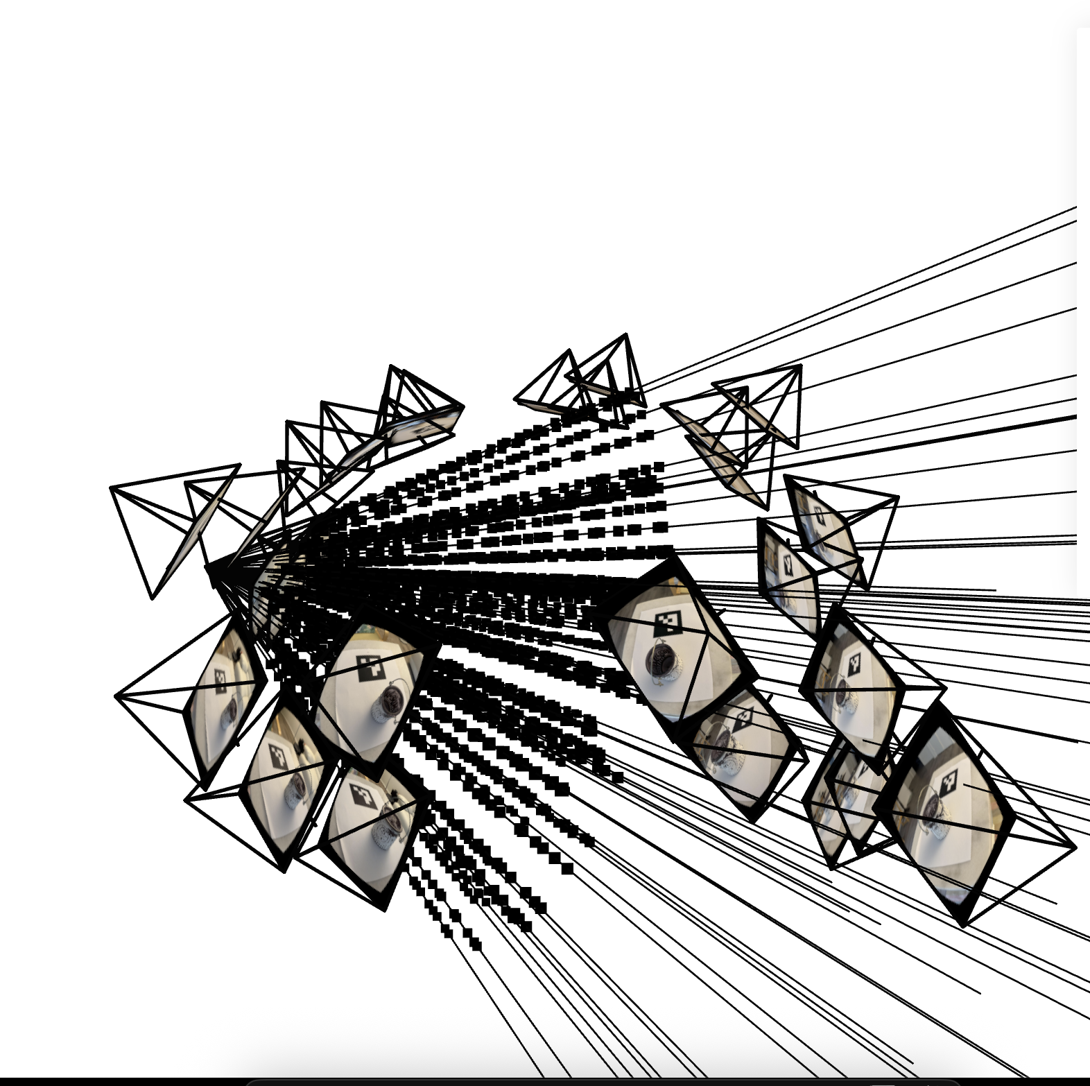
<p>We also take photos of the camera setup <em>without the object in frame</em>. This is important because it allows us to recover the camera intrinsics. Once we have the camera intrinsics and a bunch of photos of our object, 
we pass it into a method that undistorts the images, computes camera-to-world (<code class="language-plaintext highlighter-rouge">c2w</code>) matrices, and splits the photos into train, test, and validation images.</p>

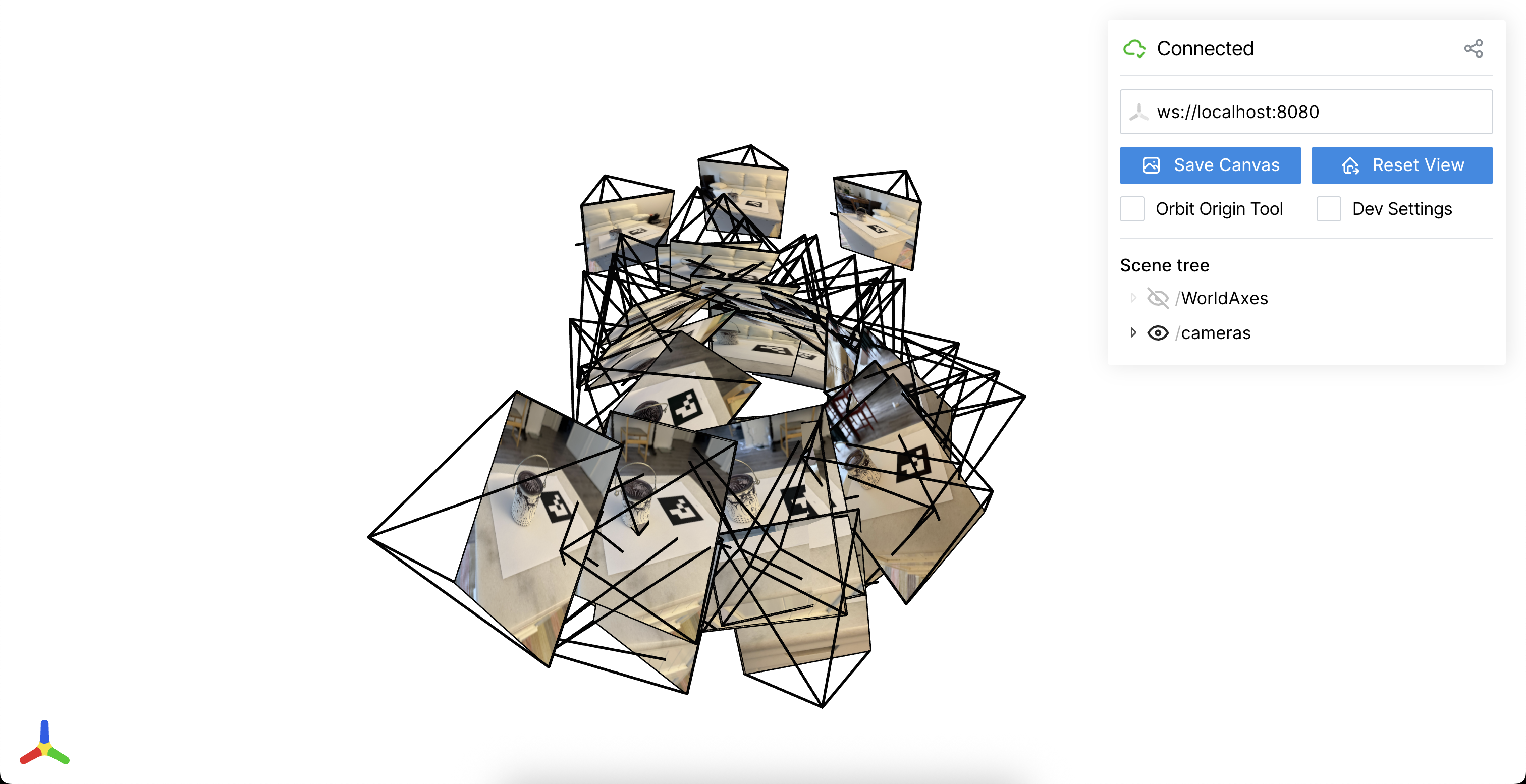
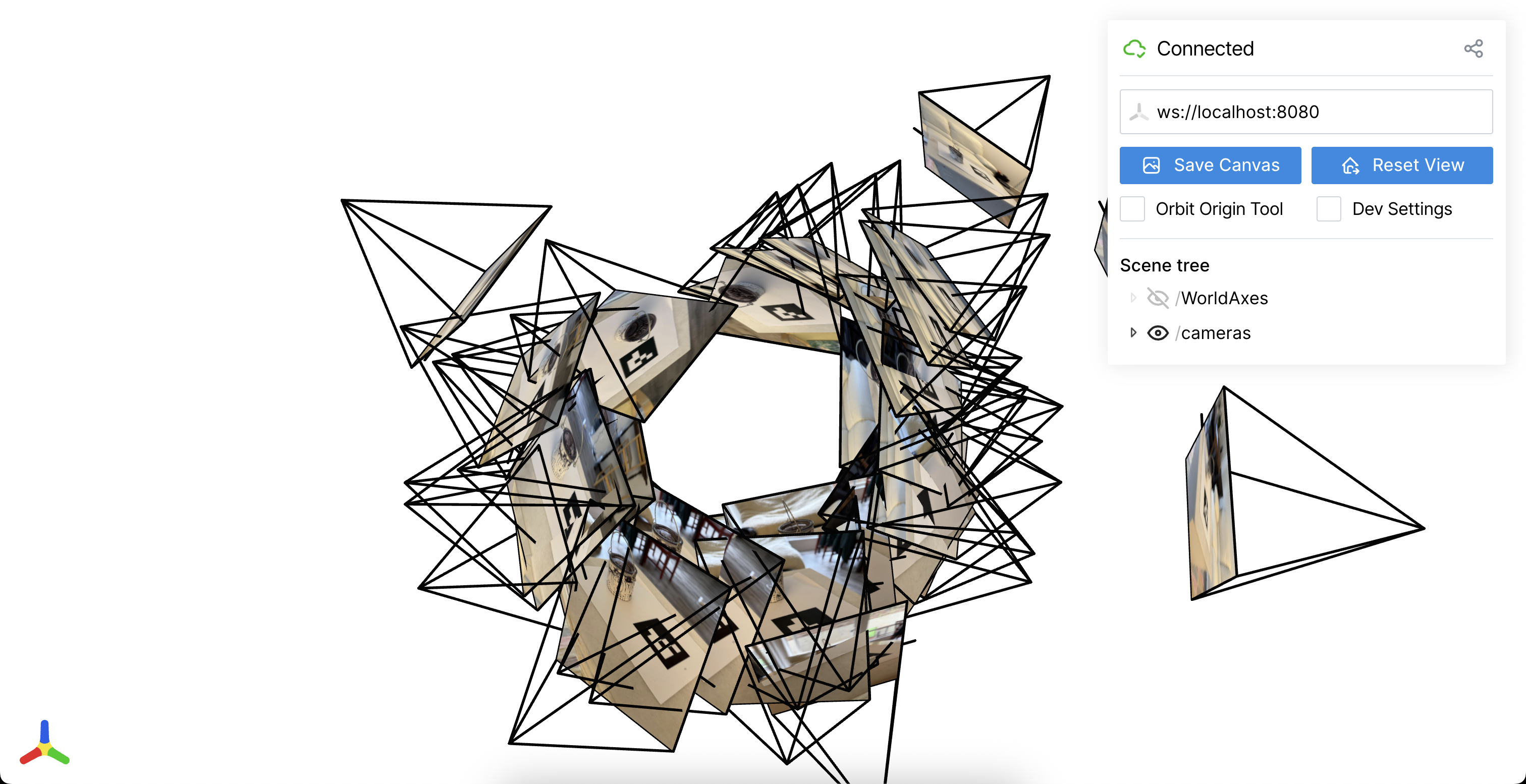
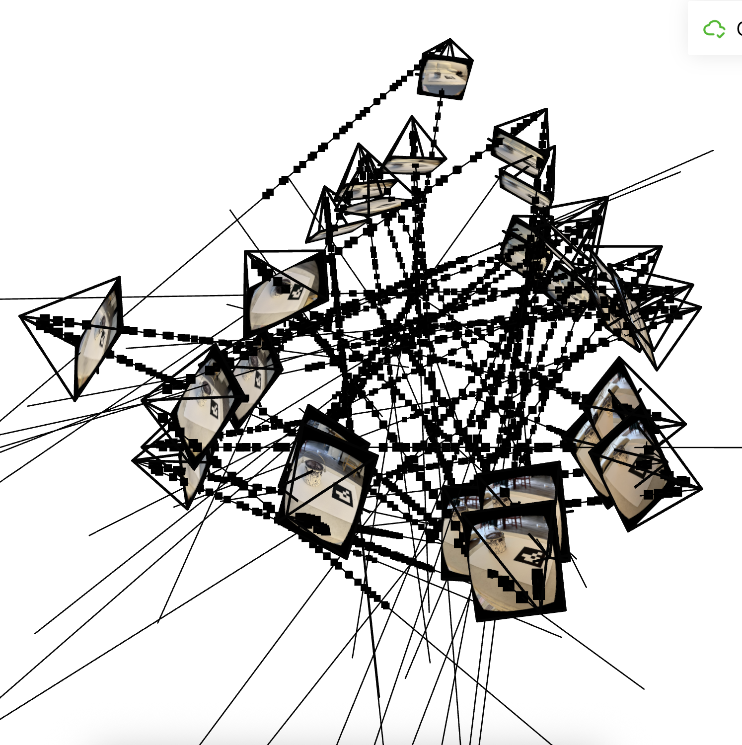
<p>Here is a visualization of the camera frustums recovered by my code from two different angles:</p>

<p align="center">
  <img src="/assets/images/nerf/visual1.png" width="1000" alt="Camera frustums view 1" />
</p>
<p align="center">
  <img src="/assets/images/nerf/visual2.png" width="1000" alt="Camera frustums view 2" />
</p>

<p>One thing I’d like to note is that setting the tag length to 60mm, which is its actual length, does not give good results because the markers end up too far apart. 
For this reason, my code assumes <code class="language-plaintext highlighter-rouge">tag_length = 0.6</code> instead of <code class="language-plaintext highlighter-rouge">tag_length = 60</code>.</p>

<h1 id="part-1-fitting-a-neural-field-to-a-2d-image">Part 1: Fitting a Neural Field to a 2D Image</h1>

<p>Our first, warmup task is to fit a neural field to a 2D image.
This isn’t used to create our NeRFs, but it’s a helpful exercise to get us familiar with the libraries
that we will be using in part 2. 
If you can understand the 2D case well, then it’s easier to generalize to 3D.
For the single-image regression task I kept the starter MLP that predicts RGB values from positional encodings of <code class="language-plaintext highlighter-rouge">(x, y)</code> coordinates.</p>

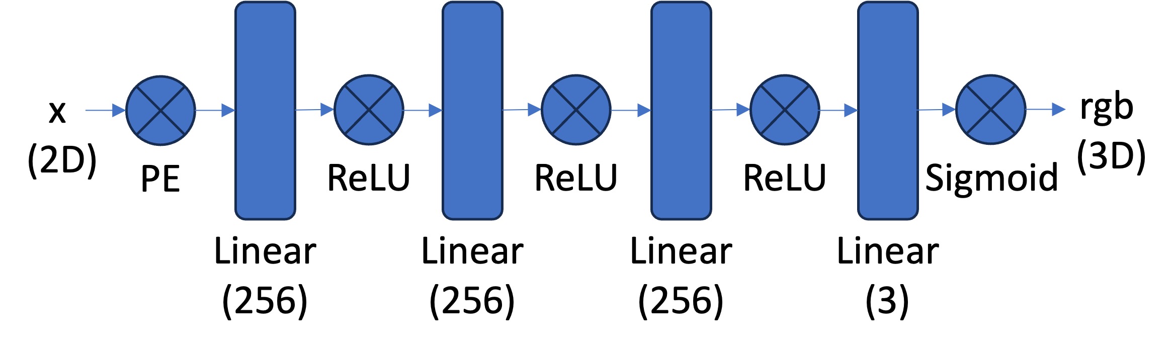
<p>This is the model architecture:</p>

<p align="center">
  <img src="/assets/images/nerf/2d_arch.jpg" alt="2D NeRF Architecture" />
</p>

<p>I trained my network using Adam as the optimizer with a learning rate of <code class="language-plaintext highlighter-rouge">1e-2</code> for 1,000 iterations with a batch size of 10k, as stated in the assignment instructions.</p>

<p>All other hyperparameters were the same as the ones described in the spec.</p>

<p>I also evaluate PSNR every 50 iterations and put that in a separate graph which you will see later in the post.</p>

<h2 id="training-progression">Training progression</h2>

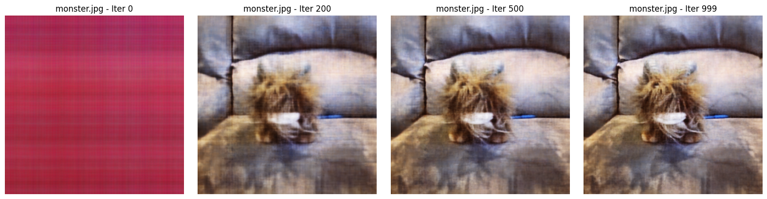
<p>The provided “monster” target converges quickly.
This makes sense, as the image was relatively simple to begin with.</p>

<p align="center">
  <img src="/assets/images/nerf/pt1/progression_monster.png" alt="Training progression on the provided monster image" />
</p>

<p>The fox image shows a similar pattern:</p>

<p align="center">
  <img src="/assets/images/nerf/pt1/progression_woof.png" alt="Training progression on my custom fox illustration" />
</p>

<h2 id="effect-of-positional-encoding-frequency-and-width">Effect of positional encoding frequency and width</h2>

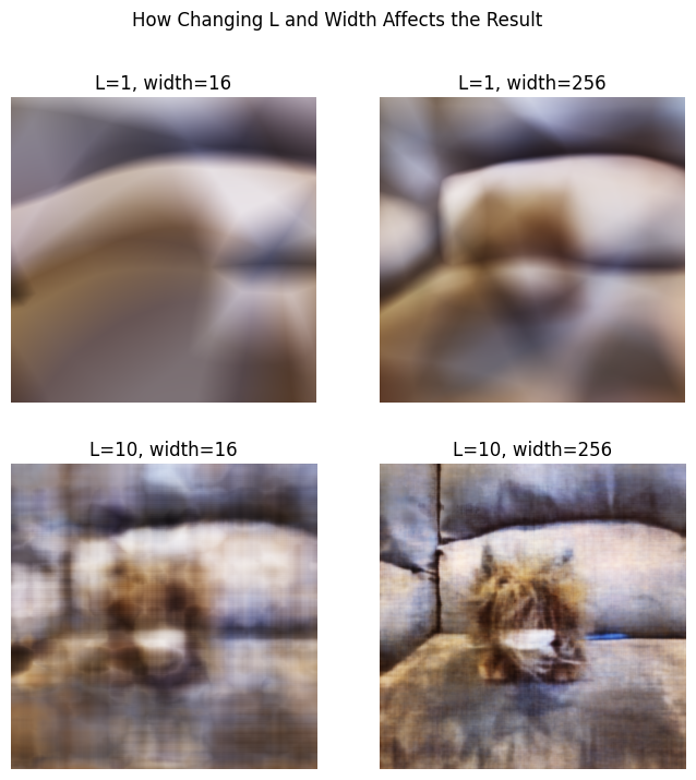
<p>Here we try various values of <em>L</em> and the hidden layer width and put them in a 2x2 grid.
This helps us understand how varying the hyperparams affects the overall predictions of the model.</p>

<p align="center">
  <img src="/assets/images/nerf/pt1/hyperparameter_grid.png" alt="Grid of final results across encoding frequency and network width" />
</p>

<h2 id="psnr-over-training">PSNR over training</h2>

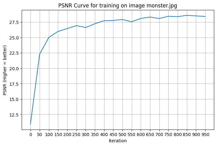
<p>The PSNR curve shows rapid gains for the first ~200 iterations. 
This makes sense because the model is learning the lower-frequency, coarse structure of the image.
Then it gets smaller improvements as it corrects the higher frequency errors.</p>

<p>Here is the PSNR curve for the custom image (<code class="language-plaintext highlighter-rouge">monster.jpg</code>):</p>

<p align="center">
  <img src="/assets/images/nerf/pt1/psnr_curve_monster.jpg.png" width="650" alt="PSNR curve for the custom image (monster.jpg) over 1000 iterations" />
</p>

<p>Overall, even this simple MLP can overfit a single view pretty well as long as you choose the right hyperparameters.</p>

<h2 id="other-notes">Other Notes</h2>

<p>One optimization that I added is that we precompute the positional encoding of all the coordinates sampled during renders.
Recall that we render a model prediction (as seen in the training progression diagram), you have to evaluate the model at many image coordinates to reconstruct its prediction.
This requires computing the <em>positional encoding</em> for each coordinate. 
But since these positional encodings are not learned parameters, we can compute the positionally-encoded version of every pixel in the render ahead of time, which speeds things up a bit.</p>

<p>There are definitely more optimizations we could have done for this part, but as Part 1 is not the main focus on the assignment, I moved on as soon as I got it to work with a reasonable runtime.</p>

<h1 id="part-2-fitting-a-neural-radiance-field-from-multi-view-images">Part 2: Fitting a Neural Radiance Field from Multi-view Images</h1>

<h2 id="how-i-implemented-each-part">How I implemented each part</h2>

<p>With the calibrated cameras from Part 0 in hand, I reconstructed a full NeRF volume for the Lego scene.</p>

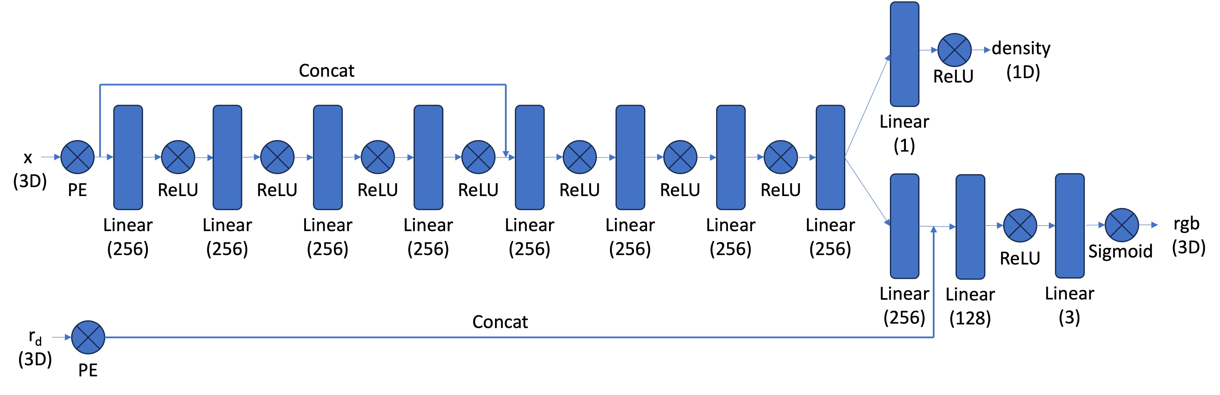
<p>Here is the architecture that I used for my neural network, as per the assignment spec:</p>

<p align="center">
  <img src="/assets/images/nerf/3d_arch.png" alt="3D NeRF Architecture" />
</p>

<p><strong>Parameters</strong>: The layers and activation functions are all the same as the architecture described in the spec. I set the positional encoding for the X dimension to have L=10, and for the depth r_d, to L=4</p>

<h3 id="vectorized-code">Vectorized Code</h3>
<p>I feel like the most crucial part of this section is correctly implementing the core methods: volumetric rendering, sampling points along rays, etc: implement these methods correctly and the training loop is generally straightforward (and doesn’t take too much added code).</p>

<p>At first I implemented some of these methods with numpy, but I found that this made training too slow and was too complicated. It required moving too many objects back and forth between my MPS backend and the CPU.</p>

<p>Instead, I implemented all the methods for sampling, dataloading, etc. in PyTorch, and I added support for batched operations. 
This made my implementation cleaner and easier to understand and debug.</p>

<h2 id="dataloader-class">Dataloader Class</h2>
<p>I also found it helpful to create a Dataloader class to abstract away some of the complexities of sampling rays from images.
My dataloader init’s method precomputes ray origins and directions for pixels <code class="language-plaintext highlighter-rouge">u, v</code> in each image.
This is similar to what we did in part 1: it speeds up training and cuts down on redundant computations.</p>

<h2 id="other-abstractions">Other Abstractions</h2>
<p>I created helper methods such as <code class="language-plaintext highlighter-rouge">nerf_forward_pass</code>, <code class="language-plaintext highlighter-rouge">render_full_image</code> and <code class="language-plaintext highlighter-rouge">make_renders</code> and housed them in a separate file called <code class="language-plaintext highlighter-rouge">pt2_utils.py</code>.
Given the overall complexity of this project, I found it necessary to separate the code into multiple files and maintain helper methods to avoid code repetition.</p>

<h2 id="visualizing-rays-and-samples">Visualizing rays and samples</h2>

<p>As per the assignment spec, I visualize rays and sample points as a sanity check to make sure my code worked:</p>

<p align="center">
  <img src="/assets/images/nerf/pt2/many_camera.png" alt="Example camera frustum and sampled rays" />
</p>

<p>Here is a visualization for just one camera:</p>
<p align="center">
  <img src="/assets/images/nerf/pt2/one_camera.png" alt="Example camera frustum and sampled rays with dots indicating the points of sampling" />
</p>

<p>where the darker dots along the lines represent points at which we sample.</p>

<p>As mentioned, we insert a small amount of noise to the sampling intervals in order to improve the model’s predictions.
This is somewhat noticeable in the visualizations above; the gap between individual sampling points is not perfectly constant - and that’s by design.</p>

<h2 id="training-progression-1">Training progression</h2>

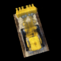
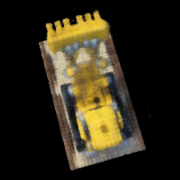
<p>The snapshots below capture the predicted RGB image for a validation camera every ~200 iterations.</p>

<div style="display: grid; grid-template-columns: repeat(3, 1fr); gap: 12px; text-align: center;">
  <figure>
    <img src="/assets/images/nerf/pt2/lego/step0.png" alt="Iteration 0 reconstruction" style="width:100%;" />
    <figcaption>Iteration 0</figcaption>
  </figure>

  <figure>
    <img src="/assets/images/nerf/pt2/lego/step99.png" alt="Iteration 99 reconstruction" style="width:100%;" />
    <figcaption>Iteration 99</figcaption>
  </figure>

  <figure>
    <img src="/assets/images/nerf/pt2/lego/step199.png" alt="Iteration 199 reconstruction" style="width:100%;" />
    <figcaption>Iteration 199</figcaption>
  </figure>

  <figure>
    <img src="/assets/images/nerf/pt2/lego/step499.png" alt="Iteration 499 reconstruction" style="width:100%;" />
    <figcaption>Iteration 499</figcaption>
  </figure>

  <figure>
    <img src="/assets/images/nerf/pt2/lego/step799.png" alt="Iteration 799 reconstruction" style="width:100%;" />
    <figcaption>Iteration 799</figcaption>
  </figure>

  <figure>
    <img src="/assets/images/nerf/pt2/lego/step999.png" alt="Iteration 999 reconstruction" style="width:100%;" />
    <figcaption>Iteration 999</figcaption>
  </figure>
</div>

<h2 id="validation-curve">Validation curve</h2>

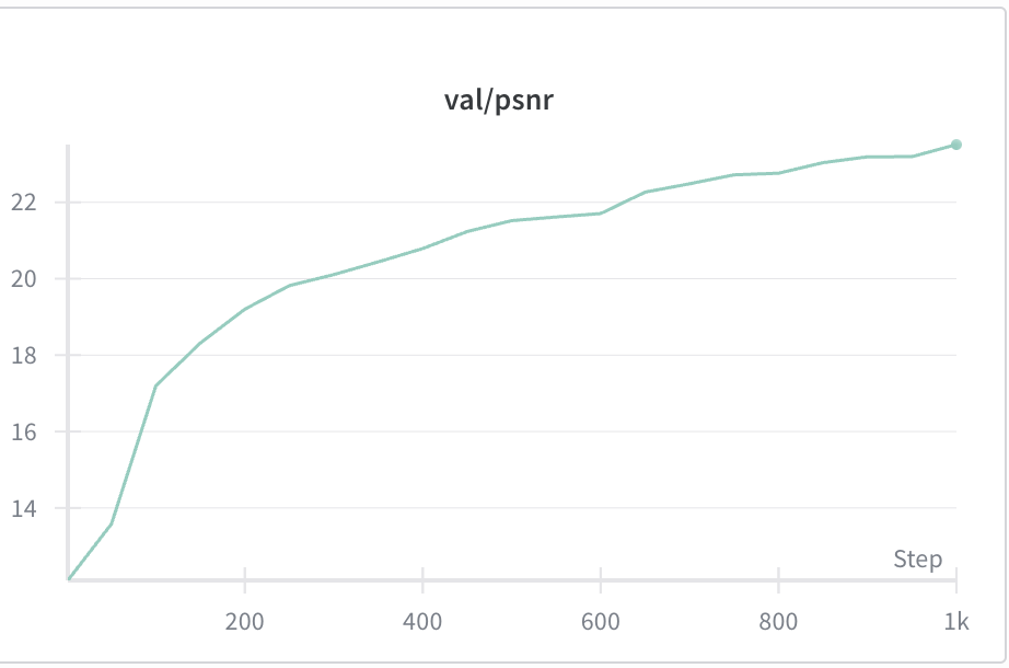
<p>I average the PSNR across six validation images to compute the <em>validation PSNR</em>.</p>

<p>The final PSNR that I achieved was <strong>23.51</strong>.</p>

<p>Here is the PSNR curve on that validation set:</p>

<p align="center">
  <img src="/assets/images/nerf/psnr_lego.png" alt="PSNR Curve on LEGO" />
</p>

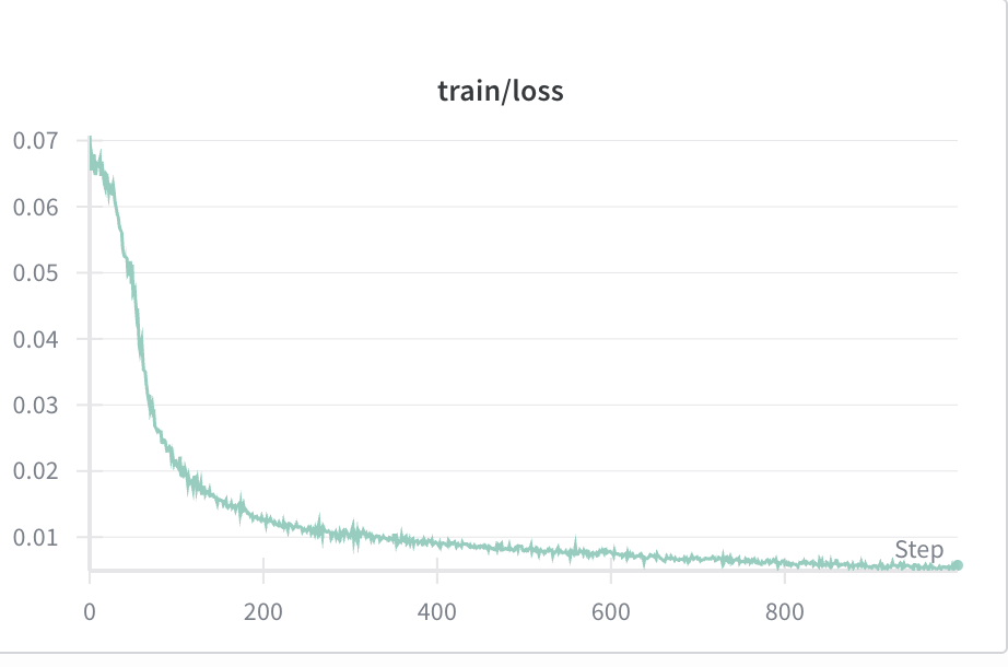
<p>Here’s the training loss curve too:</p>

<p align="center">
  <img src="/assets/images/nerf/loss_lego.png" alt="Loss Curve on LEGO" />
</p>

<h2 id="spherical-rendering">Spherical rendering</h2>

<p>After convergence I evaluate the network across a 360 degree camera path using the provided rendering code.
I use a held-out C2W matrix from the test split (<code class="language-plaintext highlighter-rouge">c2ws_test</code>) for this part.</p>

<p>Here is my spherical rendering:</p>

<p align="center">
  <img src="/assets/images/nerf/pt2/lego/final_gif.gif" alt="360 degree render of the Lego scene" />
</p>

<p>If the rendering isn’t showing, you can also view it at this link:
<a href="https://www.vkethana.com/assets/images/nerf/pt2/lego/final_gif.gif">https://www.vkethana.com/assets/images/nerf/pt2/lego/final_gif.gif</a></p>

<p>Honestly, I thought the results were pretty good given the limited amount of compute / train time we used for this assignment!</p>

<h1 id="training-with-my-own-data-part-26">Training with my own data (Part 2.6)</h1>

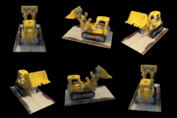
<p>After succeeding on the LeGO image, I moved on to making a NeRF with my own set of images.</p>

<p>Unfortunately, this part of the assignment did not go as well :(</p>

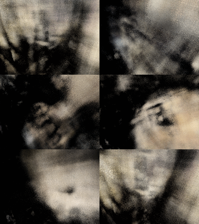
<p>Here is the best spherical rendering that I could achieve:</p>

<p align="center">
  <img src="/assets/images/nerf/pt2/my_data/final_gif.gif" alt="360 degree render of my scene" />
</p>

<p>If the rendering isn’t showing, you can also view it at this link:
<a href="https://www.vkethana.com/assets/images/nerf/pt2/my_data/final_gif.gif">https://www.vkethana.com/assets/images/nerf/pt2/my_data/final_gif.gif</a></p>

<p>The model definitely learned <em>something</em>, and you can kind of make out distinct features of the scene in which I took the images, but overall, I would say it was unsuccessful.</p>

<h2 id="training-and-psnr-plots">Training and PSNR Plots</h2>

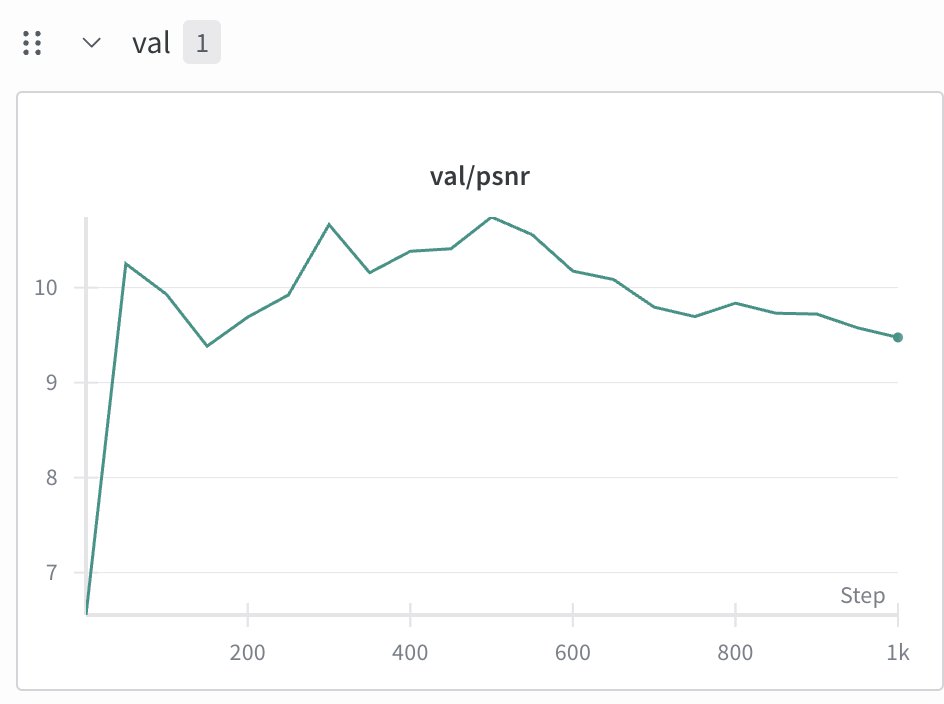
<p>Here is my PSNR curve, which reached a maximum of value of <code class="language-plaintext highlighter-rouge">10.74</code> during training.</p>

<p align="center">
  <img src="/assets/images/nerf/psnr_my_data.png" alt="PSNR Curve for my image" />
</p>

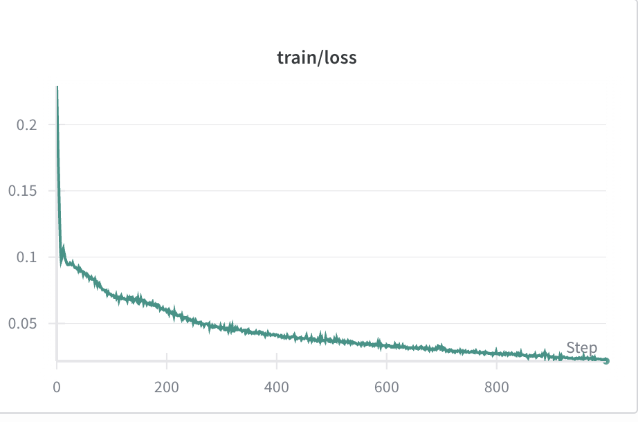
<p>On the bright side, the model did at least show convergence as seen in the below training loss graph:</p>

<p align="center">
  <img src="/assets/images/nerf/loss_my_data.png" alt="Loss curve on my data" />
</p>

<p>This suggests that the loss landscape just wasn’t shaped properly, i.e. that we need to take better photos or change something about the model architecture.</p>

<h2 id="training-progression-2">Training progression</h2>

<p>The snapshots below capture the predicted RGB image for a validation camera every ~200 iterations.</p>

<div style="display: grid; grid-template-columns: repeat(3, 1fr); gap: 12px; text-align: center;">
  <figure>
    <img src="/assets/images/nerf/pt2/my_data/step0.png" alt="Iteration 0 reconstruction" style="width:100%;" />
    <figcaption>Iteration 0</figcaption>
  </figure>

  <figure>
    <img src="/assets/images/nerf/pt2/my_data/step99.png" alt="Iteration 99 reconstruction" style="width:100%;" />
    <figcaption>Iteration 99</figcaption>
  </figure>

  <figure>
    <img src="/assets/images/nerf/pt2/my_data/step299.png" alt="Iteration 299 reconstruction" style="width:100%;" />
    <figcaption>Iteration 299</figcaption>
  </figure>

  <figure>
    <img src="/assets/images/nerf/pt2/my_data/step499.png" alt="Iteration 499 reconstruction" style="width:100%;" />
    <figcaption>Iteration 499</figcaption>
  </figure>

  <figure>
    <img src="/assets/images/nerf/pt2/my_data/step799.png" alt="Iteration 799 reconstruction" style="width:100%;" />
    <figcaption>Iteration 799</figcaption>
  </figure>

  <figure>
    <img src="/assets/images/nerf/pt2/my_data/step999.png" alt="Iteration 999 reconstruction" style="width:100%;" />
    <figcaption>Iteration 999</figcaption>
  </figure>
</div>

<h2 id="code--hyperparameter-changes-made">Code / Hyperparameter changes made</h2>
<ul>
  <li>I downsized my images from 1500 by 2000 to 150 by 200 in order to prevent OOM errors and speed up training.</li>
  <li>Recall that the original LEGO images were 200x200, so it makes sense for these images to be in roughly the same neighborhood of size</li>
  <li>I use a different set of hyperparameters: I set the positional encoding for <code class="language-plaintext highlighter-rouge">X</code> to have L = 40 and the positional encoding for <code class="language-plaintext highlighter-rouge">d</code> to have L = 15. I chose these experimentally.</li>
  <li>Additionally, I set <code class="language-plaintext highlighter-rouge">near</code> and <code class="language-plaintext highlighter-rouge">far</code> (which determine the distances at which we sample points on the rays) to <code class="language-plaintext highlighter-rouge">0.1</code> and <code class="language-plaintext highlighter-rouge">2.0</code> respectively. I made this change by looking at the rays/frustum visualization and trying different values until the length / spacing of the sampled points looked reasonable.</li>
</ul>

<h2 id="speculation-on-why-my-model-didnt-work-for-the-custom-image-the-data">Speculation on why my model didn’t work for the custom image: The Data</h2>

<p>My guess for why the model did not work very well is that the input images simply weren’t good enough: I could have taken photos from more angles to remediate this.</p>

<p>Additionally, I think it would have been good to shoot images that were closer up, given the small size of the object.</p>

<p>Using a small, black-and-white object may have also been a mistake, because many other objects in the scene were white:</p>

<ul>
  <li>the white tabletop that I placed it on</li>
  <li>the white piece of paper beneath it</li>
  <li>the white wall / couch in the background of some of the images</li>
</ul>

<h1 id="conclusion">Conclusion</h1>
<p>One key takeaway I got from the project was the importance of datasets in machine learning. The model architecture here was relatively straightforward to implement based on the assignment instructions. 
Most of the debugging effort went toward the dataloader and the sampling algorithms, not the model itself.
Ultimately, I believe it was the dataset and not the model architecture that determined the performance of the NeRF on the images that I took.</p>

<p>Overall, this was a time consuming and challenging project, but it was rewarding and taught me a lot about computer vision and implementing ML models in practice.</p>

<hr />
<div class="footnotes" role="doc-endnotes">
  <ol>
    <li id="fn:fn-1" role="doc-endnote">
      <p>I don’t reproduce my code in this blog post, as per class policies. <a href="#fnref:fn-1" class="reversefootnote" role="doc-backlink">&#8617;</a></p>
    </li>
  </ol>
</div>]]></content><author><name>Vijay Kethanaboyina</name></author><category term="machine learning" /><category term="school project" /><summary type="html"><![CDATA[TLDR]]></summary></entry><entry><title type="html">Generating Image Mosaics (without machine learning!)</title><link href="https://www.vkethana.com/mosaic/" rel="alternate" type="text/html" title="Generating Image Mosaics (without machine learning!)" /><published>2025-10-08T00:00:00+00:00</published><updated>2025-10-08T00:00:00+00:00</updated><id>https://www.vkethana.com/mosaic</id><content type="html" xml:base="https://www.vkethana.com/mosaic/"><![CDATA[<h1 id="introduction">Introduction</h1>
<p>This is my third project for CS 180 (Intro to Computer Vision) at UC Berkeley.
The project covers image warping, image mosaic generation, and automatic feature detection for image stitching.</p>

<h1 id="part-a1-shoot-the-pictures">Part A.1: Shoot the Pictures</h1>
<p>The first part of the assignment is to show at least 2 sets of images with projective transformations between them (fixed center of projection, rotate camera).
The reason we are doing this is because we can then use these images to construct mosaics later on in the assignment.</p>

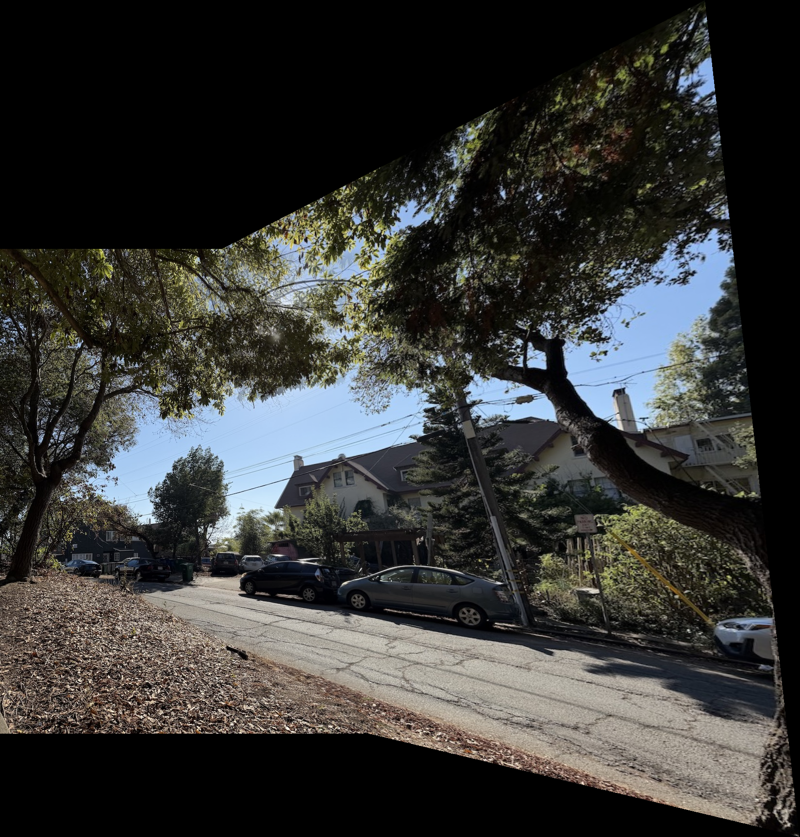
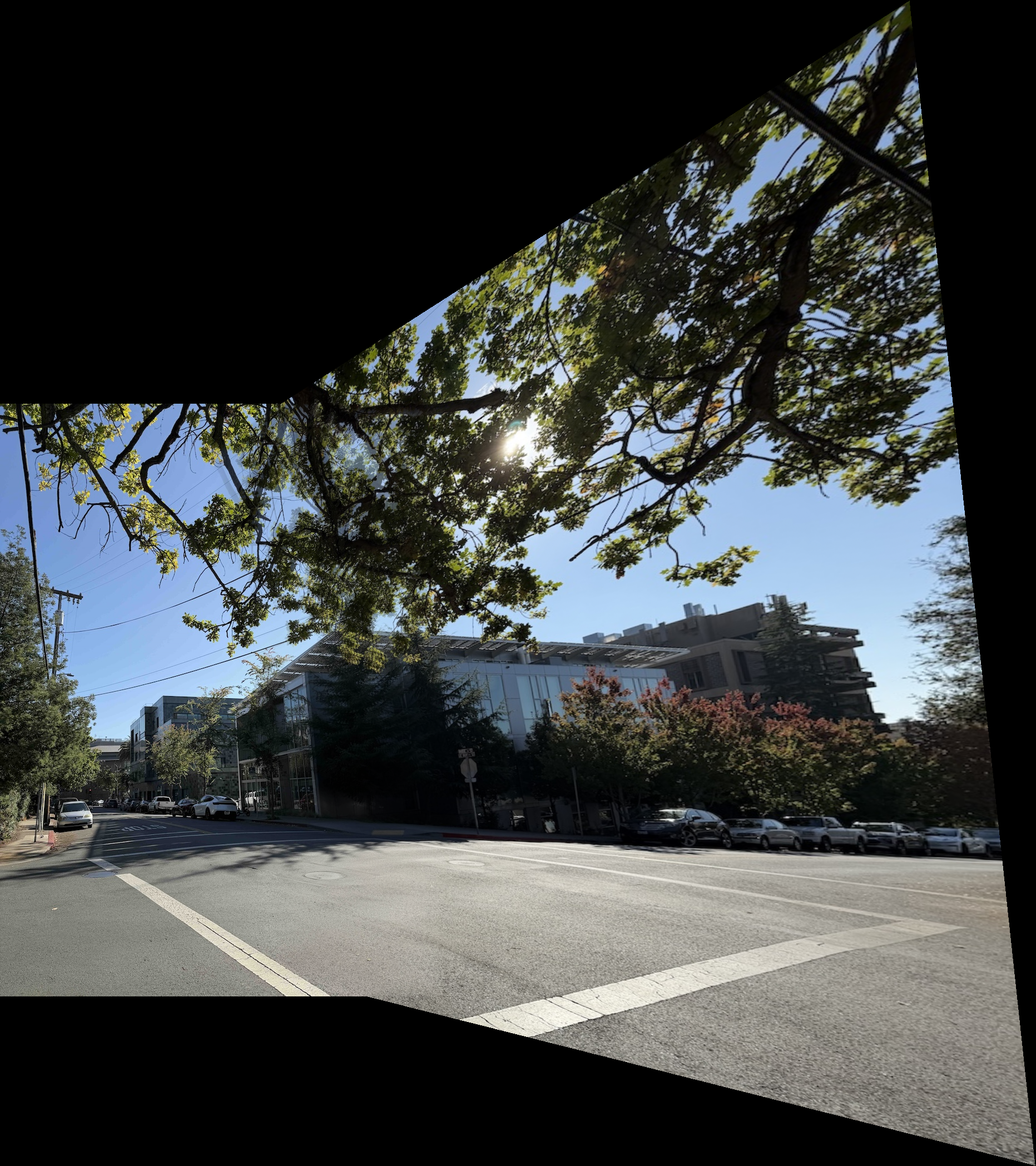
<p><strong>Set 1:</strong></p>
<p align="center">
  <img src="/assets/images/mosaic/input/northside1.jpg" width="500" />
</p>

<p align="center">
  <img src="/assets/images/mosaic/input/northside2.jpg" width="500" />
</p>

<p><strong>Set 2:</strong></p>
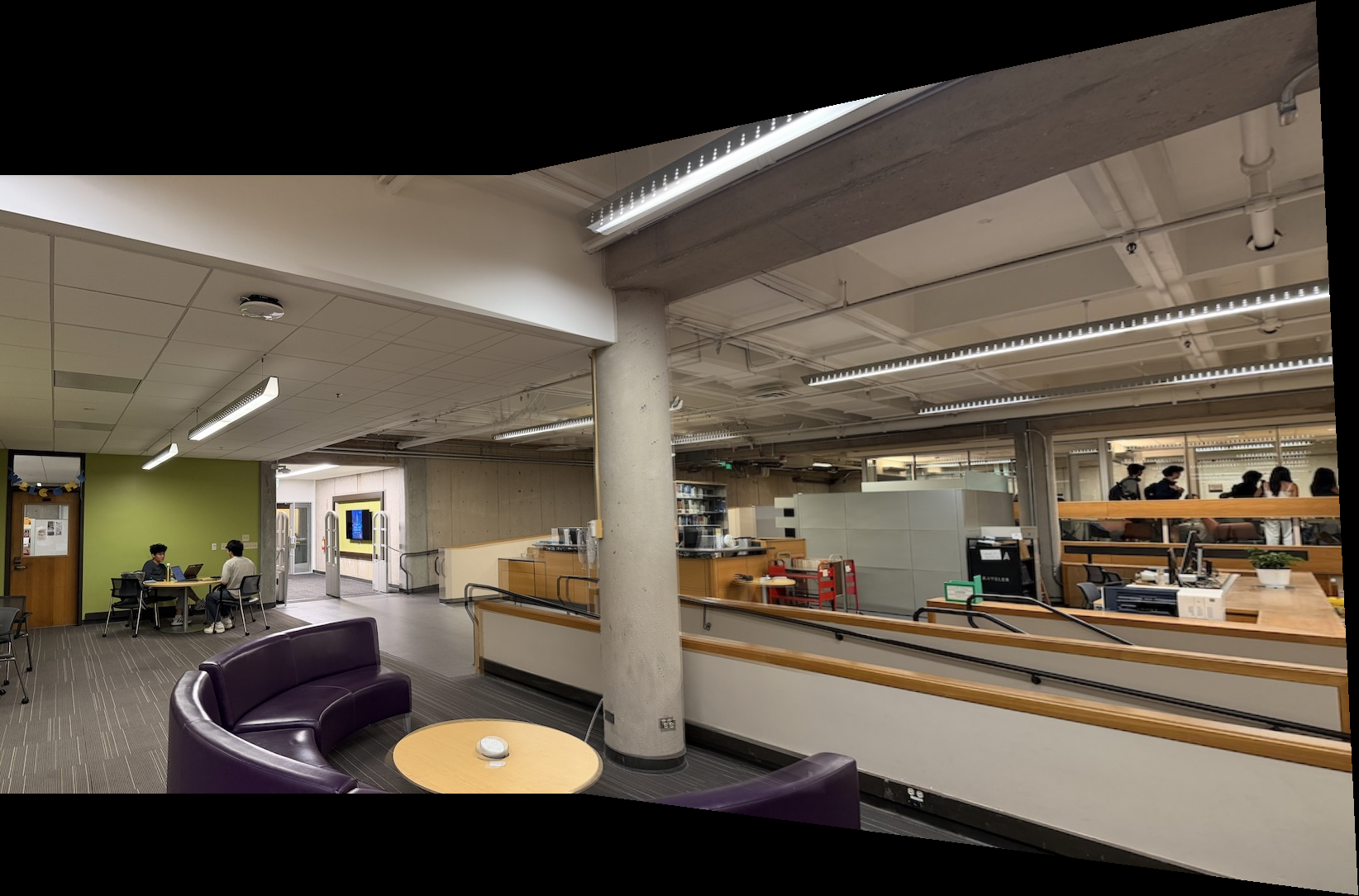
<p align="center">
  <img src="/assets/images/mosaic/input/library1.jpg" width="500" />
</p>
<p align="center">
  <img src="/assets/images/mosaic/input/library2.jpg" width="500" />
</p>

<p>Notice how the camera <em>position</em> is the same in both sets of images; all we’re doing is rotating it.
Eventually, we will stitch these images together to create an <em>image mosaic</em> (see part A.4!).</p>

<h1 id="part-a2-recover-homographies">Part A.2: Recover Homographies</h1>

<p>A <strong>homography</strong> is a 3x3 projective transformation that maps points from one image to another when both images capture the same scene.</p>

<p>For this exercise, consider the below two images:</p>

<p align="center">
  <img src="/assets/images/mosaic/output/library_compare.jpeg" width="500" />
</p>

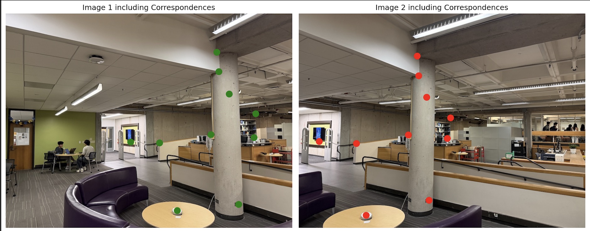
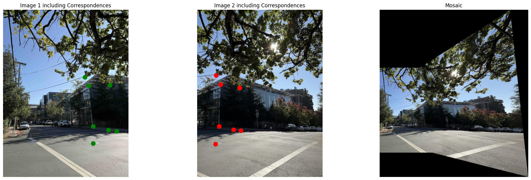
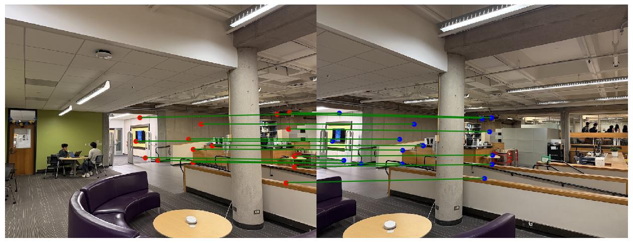
<p>Observe that I manually selected <strong>correspondence points</strong> between the two images.
These are necessary to align the images properly.
Only four points are strictly necessary for the algorithm to work, but in practice it makes sense to select many more than four for redundancy.</p>

<p>In homogeneous coordinates: <code class="language-plaintext highlighter-rouge">p2 = Hp1</code>, 
where <code class="language-plaintext highlighter-rouge">p1 = [x, y, 1]^T</code>, <code class="language-plaintext highlighter-rouge">p2 = [x', y', w']^T</code>, and <code class="language-plaintext highlighter-rouge">H</code> is:</p>

<div class="language-plaintext highlighter-rouge"><div class="highlight"><pre class="highlight"><code>[ h11 h12 h13
h21 h22 h23
h31 h32 h33 ]
</code></pre></div></div>

<p>We convert the system to Cartesian coordinates by dividing by the ‘scaling factor’ introduced by the Homogeneous coordinates:</p>

<div class="language-plaintext highlighter-rouge"><div class="highlight"><pre class="highlight"><code>x' = (h11*x + h12*y + h13) / (h31*x + h32*y + h33)
y' = (h21*x + h22*y + h23) / (h31*x + h32*y + h33)
</code></pre></div></div>
<p>Rearranging gives two equations per correspondence:</p>
<div class="language-plaintext highlighter-rouge"><div class="highlight"><pre class="highlight"><code>x*h11 + y*h12 + 1*h13 - x*x'*h31 - y*x'*h32 = x'*h33
x*h21 + y*h22 + 1*h23 - x*y'*h31 - y*y'*h32 = y'*h33
</code></pre></div></div>

<p>Setting <code class="language-plaintext highlighter-rouge">h33</code> to 1 as discussed in class, <strong>we arrive at the system of equations:</strong></p>

<div class="language-plaintext highlighter-rouge"><div class="highlight"><pre class="highlight"><code>x' = x*h11 + y*h12 + 1*h13 - x*x'*h31 - y*x'*h32 
y' = x*h21 + y*h22 + 1*h23 - x*y'*h31 - y*y'*h32 
</code></pre></div></div>

<p>Stacking all pairs yields the linear system <code class="language-plaintext highlighter-rouge">Ah = b</code> with<br />
<code class="language-plaintext highlighter-rouge">h = [h11 h12 h13 h21 h22 h23 h31 h32]^T</code>.
I solved the resulting system of equations using least-squares (because we have &gt;4 correspondences, the system is overdetermined).</p>

<p>This is the <strong>homography matrix H</strong> which I recovered:</p>
<div class="language-plaintext highlighter-rouge"><div class="highlight"><pre class="highlight"><code>[[ 1.46568340e+00 -1.20053461e-01 -4.98410322e+02]
[ 2.29064746e-01  1.24290079e+00 -1.30462059e+02]
[ 5.01352998e-04 -9.85491138e-05  1.00000000e+00]]
</code></pre></div></div>

<h1 id="part-a3-image-warping-and-rectification">Part A.3: Image Warping and Rectification</h1>

<p>In this section, I use the recovered homography <strong>H</strong> to warp images toward a reference view using <strong>inverse warping</strong>.<br />
Inverse warping maps each pixel in the <em>output</em> image back into the <em>input</em> image coordinate system.
This prevents holes or “gaps” in the outputted image.</p>

<hr />

<h2 id="1-warp-functions">1) Warp Functions</h2>
<p>After we inverse-warp the image, there’s a problem: the resulting coordinate values are not integers!
There are many kinds of interpolation methods we can apply to address this problem.
Here I discuss two interpolation methods that I implemented from scratch.</p>

<p><strong>Nearest Neighbor Interpolation</strong>: Round coordinates to the nearest pixel value. Runs relatively quickly but the results aren’t as good as bilinear interpolation.</p>

<p><strong>Bilinear Neighbor Interpolation</strong>: Use a weighted average of four neighboring pixels. Takes longer but gives better-quality results.</p>

<h2 id="2-results">2) Results</h2>
<p>In the below image, zoom in on the words “vegetarian” and “vegan” on the sign. 
Notice how the bordering around the letters is less jagged and pixelated in the bilinear interpolation image, compared to nearest-neighbor.</p>

<p align="center">
  <img src="/assets/images/mosaic/output/sign_rectification.png" width="800" />
</p>

<p>Here’s another example:</p>

<p align="center">
  <img src="/assets/images/mosaic/output/campanile_rectification.png" width="800" />
</p>

<p>For these examples, there is no ‘‘second image’’: instead, we warp the first image to a predetermined shape (a rectangle).</p>

<p>For the campanile example, I set the second image’s coordinates to that of a rectangle with height four times that of the width. Here’s what the coordinates of that rectangle looked like, for reference:</p>
<div class="language-plaintext highlighter-rouge"><div class="highlight"><pre class="highlight"><code>  "im2Points": [
    [0, 0],
    [1, 0],
    [1, 4],
    [0, 4]
  ]
</code></pre></div></div>

<p>For the sign image, I used a rectangle with height 1.58 times the width.
I determined these values through manual measurement of the image and trial and error.</p>

<h1 id="part-a4-blend-the-images-into-a-mosaic">Part A.4 Blend the Images into a Mosaic</h1>

<p>In this next part, I developed an algorithm to stitch images together into panoramas!</p>

<h2 id="procedure-one-shot-inverse-warping">Procedure (one-shot, inverse warping)</h2>

<ol>
  <li>
    <p><strong>Choose reference:</strong>
Leave one image unwarped and warp the other into its projection using the computed homography.</p>
  </li>
  <li>
    <p><strong>Create alpha masks:</strong>
For each image, define an <strong>alpha mask</strong> that indicates which pixels are valid, post-warping.</p>

    <ul>
      <li>Pixels filled during warping are set to <code class="language-plaintext highlighter-rouge">1</code> (valid).</li>
      <li>Empty or outside regions remain <code class="language-plaintext highlighter-rouge">0</code>.
These masks tell you which parts of the canvas belong to which image, and they decide how blending works in areas where the images overlap.</li>
    </ul>
  </li>
  <li>
    <p><strong>Apply weighted averaging to reduce artifacts:</strong>
To smooth the overlap between the two images, I gave each pixel a weight based on how far it is from the image edge.
To accomplish this, I define variables <code class="language-plaintext highlighter-rouge">weight_1</code> and <code class="language-plaintext highlighter-rouge">weight_2</code>, where each is computed from the <strong>distance transform</strong> of its image’s alpha mask:</p>
    <div class="language-plaintext highlighter-rouge"><div class="highlight"><pre class="highlight"><code>dist_1 = distance_transform_edt(alpha_mask_1) # distance transform method imported from scipy
weight_1 = dist_1 / (np.max(dist_1) + 1e-8)
# dist_2, weight_2 defined the same way
</code></pre></div>    </div>

    <p>Pixels near the center of each image have higher weights, and edge pixels have lower weights.
When blending, areas of overlap are averaged accordingly:</p>
    <div class="language-plaintext highlighter-rouge"><div class="highlight"><pre class="highlight"><code>mosaic = (weight_1 * image_1 + weight_2 * image_2) / (weight_1 + weight_2)
</code></pre></div>    </div>

    <p>This produces a soft, seamless transition between the two images.
(In practice, the averaging is applied separately to each color channel, not all at once.)</p>
  </li>
</ol>

<h2 id="results">Results</h2>

<p>Here are the mosaics with the original images:</p>
<p align="center">
  <img src="/assets/images/mosaic/output/road1_road2_mosaic_compare.png" width="800" />
</p>

<p align="center">
  <img src="/assets/images/mosaic/output/northside1_northside2_mosaic_compare.png" width="800" />
</p>

<p align="center">
  <img src="/assets/images/mosaic/output/library1_library2_mosaic_compare.png" width="800" />
</p>

<p>Here are the mosaics on their own for reference:</p>

<p align="center">
  <img src="/assets/images/mosaic/output/road1_road2_mosaic.png" width="600" />
</p>

<p align="center">
  <img src="/assets/images/mosaic/output/northside1_northside2_mosaic.png" width="600" />
</p>

<p align="center">
  <img src="/assets/images/mosaic/output/library1_library2_mosaic.png" width="600" />
</p>

<hr />

<h1 id="part-b-automatic-feature-detection-and-matching">Part B: Automatic Feature Detection and Matching</h1>

<p>In Part A, I manually selected correspondence points to create mosaics. This was tedious and error-prone.
In Part B, I implemented an automatic system that detects features, matches them between images, and creates mosaics without any manual input.</p>

<p>The algorithm is based on the paper “Multi-Image Matching using Multi-Scale Oriented Patches” by Brown et al.</p>

<h1 id="part-b1-harris-corner-detection">Part B.1: Harris Corner Detection</h1>

<p>The first step is to detect interesting points (corners) in the image automatically.
I used the Harris corner detector to find points with strong intensity gradients in multiple directions.</p>

<p>Here’s the result on a test image with all detected Harris corners:</p>

<p align="center">
  <img src="/assets/images/mosaic/output/sign_harris.jpg" />
</p>

<p>As you can see, there are way too many corners detected.</p>

<p>How can we extract the most important corners and filter out the rest? 
That’s where ANMS comes in clutch!</p>

<h2 id="adaptive-non-maximal-suppression-anms">Adaptive Non-Maximal Suppression (ANMS)</h2>

<p>We use Adaptive Non-Maximal Suppression (ANMS) to get a more uniform spatial distribution of interest points. 
Each point’s suppression radius depends on its corner strength: points are kept <em>only if</em> they are local maxima within a radius where no stronger neighbor exists. 
The minimum suppression radius for a point <code class="language-plaintext highlighter-rouge">x_i</code> is defined as the distance to the nearest point <code class="language-plaintext highlighter-rouge">x_j</code> with significantly higher strength, <code class="language-plaintext highlighter-rouge">f(x_i) &lt; c_robust * f(x_j)</code>, using <code class="language-plaintext highlighter-rouge">c_robust = 0.9</code>.</p>

<p>Here’s the same image after applying ANMS to filter the bad corners.</p>

<p align="center">
  <img src="/assets/images/mosaic/output/sign_harris_anms.jpg" />
</p>

<p>The selected corners are much more evenly distributed and correspond to distinctive features in the image.</p>

<h1 id="part-b2-feature-descriptor-extraction">Part B.2: Feature Descriptor Extraction</h1>

<p>Once I have corner locations, we need to describe what each corner looks like so we can match them between images.</p>

<p>For each corner, I extracted a 40×40 patch around it, convolved it with a Gaussian filter to blur it (using code from project 2), then downsampled it to 8×8.
I normalized each descriptor to have zero mean and unit variance, as is standard practice.</p>

<p>Here are some of the 8×8 feature descriptors I extracted.
Each small patch captures the local appearance around a corner point.</p>

<p align="center">
  <img src="/assets/images/mosaic/output/descriptor.png" />
</p>

<h1 id="part-b3-feature-matching">Part B.3: Feature Matching</h1>

<p>To match features between two images, I compared their descriptors.
For each feature in image 1, I found its closest match in image 2 by computing the distance between descriptors.</p>

<p>Of course, not all the matches are good. 
I used <strong>Lowe’s ratio test</strong> to filter out bad matches:</p>
<ul>
  <li>For each feature, find the two closest matches</li>
  <li>Keep the match only if the closest is significantly better than the second-closest</li>
  <li>Ratio threshold: if <code class="language-plaintext highlighter-rouge">distance_to_best / distance_to_second &lt; 0.85</code>, keep it</li>
</ul>

<p>The intuition here is that if you are torn between two options, chances are that neither of them are very good.
There should be <em>one option</em> that is vastly better than all the others.</p>

<p>Here are the feature matches I found between two library images:</p>

<p align="center">
  <img src="/assets/images/mosaic/output/library1_library2_feature_matches.jpg" width="800" />
</p>

<p>You might have noticed that some of these matches are not good, even with Lowe’s ratio test.
But don’t worry!
In the next subpart, we will fix this issue.</p>

<h1 id="part-b4-ransac-and-automatic-mosaics">Part B.4: RANSAC and Automatic Mosaics</h1>

<p>The code we just wrote has a problem - some feature matches are still wrong. 
We refer to this bad matches as <em>outliers</em>.
Conversely, desirable matches (ones that are correct) are called <em>inliers</em>.
We want to compute the optimal homography using just the inlier points, not the outliers. 
That’s where we use RANSAC: Random Sample Consensus, an interesting algorithm that actually has many applications beyond just image processing.</p>

<p><strong>How RANSAC Works:</strong></p>

<ol>
  <li>Randomly sample 4 feature correspondences</li>
  <li>Compute a homography from these 4 points</li>
  <li>Count how many other matches agree with this homography (or are reasonably close)</li>
  <li>Keep largest set of inliers</li>
  <li>Recompute the final homography, using just the inliers</li>
</ol>

<p>Here are the matches after RANSAC filtering (only inliers shown):</p>

<p align="center">
  <img src="/assets/images/mosaic/output/library1_library2_inlier_matches.jpg" width="800" />
</p>

<h2 id="automatic-vs-manual-mosaics">Automatic vs Manual Mosaics</h2>

<p>Now, we can create mosaics automatically, without painstakingly labeling correspondences. 
Here’s a comparison of manual stitching (Part A) versus automatic stitching (Part B) on the same image pairs:</p>

<p><strong>Library Mosaic:</strong></p>
<p align="center">
  <img src="/assets/images/mosaic/output/library1_library2_comparison.jpg" width="900" />
</p>

<p><strong>Northside Mosaic:</strong></p>
<p align="center">
  <img src="/assets/images/mosaic/output/northside1_northside2_comparison.jpg" width="900" />
</p>

<p><strong>Road Mosaic:</strong></p>
<p align="center">
  <img src="/assets/images/mosaic/output/road1_road2_comparison.jpg" width="900" />
</p>

<p>One key takeaway here is that RANSAC achieves pretty good results!
The manual mosaics are better in a few spots, but given that RANSAC doesn’t have access to the manual correspondences, I think it did well.</p>

<h1 id="what-i-learned">What I Learned</h1>

<p>The biggest takeaway I got from this project was the importance of <em>filtering heuristics</em>: algorithms / techniques for turning a large, messy set of features into something actually useful.
An example of a “filtering heuristic” would be Lowe’s ratio test, as well as ANMS. 
The intuitions behind why we filter out certain points and keep others are definitely something that generalizes beyond image processing. 
As I continue in my ML journey, I will keep in mind these broad takeaways.</p>]]></content><author><name>Vijay Kethanaboyina</name></author><category term="school project" /><summary type="html"><![CDATA[Introduction This is my third project for CS 180 (Intro to Computer Vision) at UC Berkeley. The project covers image warping, image mosaic generation, and automatic feature detection for image stitching.]]></summary></entry><entry><title type="html">Making Orapples: Fun with Filters, Frequencies, and Image Blending</title><link href="https://www.vkethana.com/frequency/" rel="alternate" type="text/html" title="Making Orapples: Fun with Filters, Frequencies, and Image Blending" /><published>2025-09-26T00:00:00+00:00</published><updated>2025-09-26T00:00:00+00:00</updated><id>https://www.vkethana.com/frequency</id><content type="html" xml:base="https://www.vkethana.com/frequency/"><![CDATA[<h1 id="tldr">TLDR</h1>
<p>This is my second project for CS 180 (Intro to Computer Vision) at UC Berkeley. The project goes over how filters work in image processing and how we can manipulate images in the frequency domain to get interesting effects like edge detection, sharpening, and multiresolution blending.
Here’s an example of a blended image I made as part of this project:</p>
<p align="center">
  <img src="/assets/images/frequency/pt2/oraple.jpg" width="400" />
</p>

<hr />

<h1 id="part-1-filters-and-edges">Part 1: Filters and Edges</h1>

<h2 id="part-11-finite-difference-operator">Part 1.1: Finite Difference Operator</h2>

<p>I implemented a zero-padded 2D convolution operation in NumPy, then compared it with <code class="language-plaintext highlighter-rouge">scipy.signal.convolve2d</code>.</p>

<h3 id="implementation-details">Implementation Details</h3>
<p>I created two versions:</p>
<ul>
  <li><strong>4-loop version</strong>: Explicitly loops through every kernel element</li>
  <li><strong>2-loop version</strong>: Uses vectorized operations like <code class="language-plaintext highlighter-rouge">np.dot</code></li>
</ul>

<p>Both implementations produce the same results though the two-loop version is more efficient. 
One difference from scipy is boundary handling: my implementation uses zero-padding, but <code class="language-plaintext highlighter-rouge">scipy.signal.convolve2d</code> has various other options (fill, wrap, symm).</p>

<h3 id="runtime-comparison">Runtime Comparison</h3>
<p>The 2-loop implementation is faster than the 4-loop version due to vectorization. 
However, <code class="language-plaintext highlighter-rouge">scipy.signal.convolve2d</code> is still much faster, probably because it utilizes advanced techniques like FFT to bring down the runtime from O(n^2) - which is my algorithm’s runtime - to O(n log n).</p>

<h3 id="code-snippets">Code Snippets</h3>
<p>Two-loop convolution:</p>
<div class="language-plaintext highlighter-rouge"><div class="highlight"><pre class="highlight"><code>def convolve(im, kernel):
    pad_x = kernel.shape[1] // 2
    pad_y = kernel.shape[0] // 2

    padded_im = np.zeros((2 * pad_y + im.shape[0], 2 * pad_x + im.shape[1]))
    padded_im[pad_y : pad_y+im.shape[0], pad_x : pad_x+im.shape[1]] = im

    kernel_flat = kernel.flatten()

    new_image = []
    for i in range(im.shape[0]):
        new_row = []
        for j in range(0,im.shape[1]):
            curr_chunk = padded_im[i : i + kernel.shape[0], j : j + kernel.shape[1]].flatten()
            new_pixel = np.dot(kernel_flat, curr_chunk)
            new_row.append(new_pixel)
        new_image.append(new_row)
    new_image = np.array(new_image)

    assert im.shape == new_image.shape, "Shape mismatch detected!"
    return new_image
</code></pre></div></div>

<p>Four-loop convolution:</p>
<div class="language-plaintext highlighter-rouge"><div class="highlight"><pre class="highlight"><code>def convolve_slow(im, kernel):
    pad_x = kernel.shape[1] // 2
    pad_y = kernel.shape[0] // 2

    padded_im = np.zeros((2 * pad_y + im.shape[0], 2 * pad_x + im.shape[1]))
    padded_im[pad_y : pad_y+im.shape[0], pad_x : pad_x+im.shape[1]] = im

    kernel_flat = kernel.flatten()

    new_image = np.zeros_like(im, dtype=float)
    for i in range(im.shape[0]):
        new_row = []
        for j in range(0,im.shape[1]):
            res = 0.0
            for m in range(kernel.shape[0]):
                for n in range(kernel.shape[1]):
                    res += kernel[m, n] * padded_im[i+m, j+n]
            new_image[i, j] = res

    assert im.shape == new_image.shape, "Shape mismatch detected!"
    return new_image
</code></pre></div></div>

<h3 id="results-finite-difference-filters">Results: Finite Difference Filters</h3>

<p>I applied finite difference operators Dx = <code class="language-plaintext highlighter-rouge">[1, 0, -1]</code> and Dy = <code class="language-plaintext highlighter-rouge">[1, 0, -1]^T</code>:</p>

<p align="center">
  <img src="/assets/images/frequency/pt1/selfie_dx.jpg" width="250" />
  <img src="/assets/images/frequency/pt1/selfie_dy.jpg" width="250" />
</p>
<p align="center"><em>Top: Dx (horizontal gradients). Bottom: Dy (vertical gradients)</em></p>

<p>I also tested a 9x9 box filter for smoothing:</p>

<p align="center">
  <img src="/assets/images/frequency/pt1/selfie_box.jpg" width="250" />
  <img src="/assets/images/frequency/pt1/selfie_box_scipy.jpg" width="250" />
</p>
<p align="center"><em>Top: My implementation (zero-padding). Bottom: Scipy (default boundary)</em></p>

<hr />

<h2 id="part-12-finite-difference-operator">Part 1.2: Finite Difference Operator</h2>

<p>Using the cameraman image, I computed partial derivatives and edge detection with finite differences.</p>

<p align="center">
  <img src="/assets/images/frequency/pt1/cameraman_dx.jpg" width="200" />
  <img src="/assets/images/frequency/pt1/cameraman_dy.jpg" width="200" />
  <img src="/assets/images/frequency/pt1/cameraman_gradient_mag.jpg" width="200" />
  <img src="/assets/images/frequency/pt1/cameraman_edge_image.jpg" width="200" />
</p>
<p align="center"><em>Partial derivatives, gradient magnitude, and binarized edges (threshold=0.20)</em></p>

<p>The edge image shows significant noise, which is why I had to apply the threshold of 0.20. 
I chose 0.20 because lower values recorded too much noise in areas like the sky, while higher values removed important edge details in areas like the tripod.
A better approach to this problem is to apply Gaussian smoothing first.</p>

<hr />

<h2 id="part-13-derivative-of-gaussian-dog-filter">Part 1.3: Derivative of Gaussian (DoG) Filter</h2>

<h3 id="background-info">Background Info</h3>
<p>To create the Gaussian kernel, I select a value of sigma, by default 2.0, and then compute the <code class="language-plaintext highlighter-rouge">ksize</code>, which I set as 6 times sigma plus one. 
I then invoke the <code class="language-plaintext highlighter-rouge">cv2.getGaussianKernel</code> with these two parameters.
In this approach, because ksize is uniquely determined by sigma, I only specify the sigma values when listing the parameters.</p>

<h3 id="method-1-gaussian--derivative">Method 1: Gaussian → Derivative</h3>

<p>First blur the image with a Gaussian, then apply finite difference operators:</p>

<p align="center">
  <img src="/assets/images/frequency/pt1/gauss_cameraman_dx.jpg" width="200" />
  <img src="/assets/images/frequency/pt1/gauss_cameraman_dy.jpg" width="200" />
  <img src="/assets/images/frequency/pt1/gauss_gradient_mag.jpg" width="200" />
  <img src="/assets/images/frequency/pt1/gauss_edge_image.jpg" width="200" />
</p>
<p align="center"><em>Gaussian blur (sigma=2.0) then derivatives (threshold=0.10) - much cleaner edges!</em></p>

<p>I chose a threshold of 0.10 by trial and error: I found that it reduced noise without removing too much valuable information.</p>

<h3 id="method-2-single-dog-convolution">Method 2: Single DoG Convolution</h3>

<p>By the property of convolution associativity, we can combine the Gaussian and derivative filters first, then apply to the image in one pass.
Using the combined DoG filter gives <strong>identical results</strong> to applying the two filters separately.
The Gaussian filter here uses sigma = 2.0 just like in method 1.</p>

<p><strong>The DoG filters:</strong></p>
<p align="center">
  <img src="/assets/images/frequency/pt1/dog_filters.png" width="600" />
</p>

<p>For example, here’s the edge image generated by the combined filter. This produces identical results to Method 1 and demonstrates the associativity property of convolution: (Image ⊗ Gaussian) ⊗ Derivative = Image ⊗ (Gaussian ⊗ Derivative).
<strong>Results:</strong></p>
<p align="center">
  <img src="/assets/images/frequency/pt1/alternate_gauss_edge_image.jpg" width="300" />
  <img src="/assets/images/frequency/pt1/alternate_gauss_gradient_mag.jpg" width="300" />
</p>

<hr />

<h1 id="part-2-applications">Part 2: Applications</h1>

<h2 id="part-21-image-sharpening">Part 2.1: Image “Sharpening”</h2>

<p>The unsharp mask filter enhances edges by emphasizing high frequencies. The process:</p>

<ol>
  <li>Blur the image to get low frequencies</li>
  <li>Subtract blurred from original to isolate high frequencies</li>
  <li>Add scaled high frequencies back: <code class="language-plaintext highlighter-rouge">sharpened = original + α × (original - blurred)</code></li>
</ol>

<h3 id="taj-mahal-results">Taj Mahal Results</h3>

<p align="center">
  <img src="/assets/images/frequency/input/taj.jpg" width="250" />
  <img src="/assets/images/frequency/pt2/blurred-taj.jpg" width="250" />
</p>
<p align="center">
  <img src="/assets/images/frequency/pt2/highfreq-taj.jpg" width="250" />
  <img src="/assets/images/frequency/pt2/sharpened-taj.jpg" width="250" />
</p>
<p align="center"><em>Original, blurred, high frequencies, and sharpened (α=2.0)</em></p>

<h3 id="varying-alpha-parameter">Varying Alpha Parameter</h3>

<p align="center">
  <img src="/assets/images/frequency/pt2/sharpened-alpha0.5-taj.jpg" width="180" />
  <img src="/assets/images/frequency/pt2/sharpened-alpha1.0-taj.jpg" width="180" />
  <img src="/assets/images/frequency/pt2/sharpened-alpha2.0-taj.jpg" width="180" />
  <img src="/assets/images/frequency/pt2/sharpened-alpha5.0-taj.jpg" width="180" />
</p>
<p align="center"><em>α = 0.5, 1.0, 2.0, 5.0 (more α = more sharpening, but also artifacts)</em></p>

<h3 id="additional-example">Additional Example</h3>

<p align="center">
  <img src="/assets/images/frequency/input/saint.jpg" width="450" />
  <img src="/assets/images/frequency/pt2/sharpened-saint.jpg" width="450" />
</p>
<p align="center"><em>Original and sharpened (α=40.0)</em></p>

<h3 id="blur--sharpen-experiment">Blur → Sharpen Experiment</h3>

<p>Can sharpening recover a blurred image?</p>

<p align="center">
  <img src="/assets/images/frequency/pt2/sharpened-taj.jpg" width="300" />
  <img src="/assets/images/frequency/pt2/sharpened-blurred-taj.jpg" width="300" />
</p>
<p align="center"><em>Original sharp vs. blurred then sharpened - some detail lost forever</em></p>

<p>Sharpening helps, but there’s no way to fully recover lost information. Blurring is irreversible.</p>

<hr />

<h2 id="part-22-hybrid-images">Part 2.2: Hybrid Images</h2>

<p>Hybrid images take advantage of how the human eye perceives frequencies at different distances. 
The technique combines the low-frequency components of one image with the high-frequency components of another. 
Low frequencies capture broad shapes and overall structure, which dominate our perception from far away. 
High frequencies encode fine details and edges, which we perceive up close. 
To create a hybrid image, I apply a Gaussian low-pass filter to extract smooth, large-scale features from the first image, then subtract a Gaussian-blurred version from the second image to obtain only its high-frequency details. 
When these are combined, viewers see different images depending on their distance from the image: the high-frequency image is seen from close up and the low-frequency one from far away.</p>

<h3 id="example-1-derek--nutmeg">Example 1: Derek + Nutmeg</h3>

<p align="center">
  <img src="/assets/images/frequency/input/man.jpg" width="250" />
  <img src="/assets/images/frequency/input/cat.jpg" width="250" />
  <img src="/assets/images/frequency/pt2/hybrid-man-cat.jpg" width="250" />
</p>

<p><strong>Frequency Analysis for this example:</strong></p>
<p align="center">
  <img src="/assets/images/frequency/pt2/fft-analysis.jpg" width="700" />
</p>

<p><strong>Filtered Results:</strong></p>
<p align="center">
  <img src="/assets/images/frequency/pt2/hybrid_low_pass.jpg" width="250" />
  <img src="/assets/images/frequency/pt2/hybrid_high_pass.jpg" width="250" />
</p>

<p>For this example, the low-pass Gaussian filter had a sigma value of 15.0 whereas the high-pass Gaussian filter had a sigma value of 6.0.
The images were already aligned well, so I performed no manual alignment.
(As for the ksize, it is determined by the formula <code class="language-plaintext highlighter-rouge">ksize = int(sigma*6.0 + 1)</code>.)</p>

<h3 id="example-2-tennis-ball--monster">Example 2: Tennis Ball + Monster</h3>

<p align="center">
  <img src="/assets/images/frequency/input/tennis.jpg" width="250" />
  <img src="/assets/images/frequency/input/small_monster.jpg" width="250" />
  <img src="/assets/images/frequency/pt2/hybrid-tennis-small_monster.jpg" width="250" />
</p>

<h3 id="example-3-dog--cat">Example 3: Dog + Cat</h3>

<p align="center">
  <img src="/assets/images/frequency/input/dog.jpg" width="250" />
  <img src="/assets/images/frequency/input/new_cat.jpg" width="250" />
  <img src="/assets/images/frequency/pt2/hybrid-dog-new_cat.jpg" width="250" />
</p>

<hr />

<h2 id="part-23-gaussian-and-laplacian-stacks">Part 2.3: Gaussian and Laplacian Stacks</h2>

<p>Gaussian stacks progressively blur images, while Laplacian stacks capture details at each frequency band.</p>

<h3 id="apple-stack-for-oraple-blending">Apple Stack (for Oraple blending)</h3>
<p align="center">
  <img src="/assets/images/frequency/pt2/gaussian-laplacian-stack-orapple-im1.jpg" width="100%" />
</p>

<h3 id="orange-stack-for-oraple-blending">Orange Stack (for Oraple blending)</h3>
<p align="center">
  <img src="/assets/images/frequency/pt2/gaussian-laplacian-stack-orapple-im2.jpg" width="100%" />
</p>

<hr />

<h2 id="part-24-multiresolution-blending">Part 2.4: Multiresolution Blending</h2>

<p>Using Laplacian stacks, we blend images seamlessly across frequency bands.</p>

<h3 id="oraple-apple--orange">Oraple (Apple + Orange)</h3>

<p><strong>Blending Process:</strong></p>
<p align="center">
  <img src="/assets/images/frequency/pt2/orapple_blending_process.png" />
</p>
<p align="center"><em>High frequencies show fine details, low frequencies show structure. Here I recreate the outcomes of Figure 3.42 from Szelski</em></p>

<p><strong>Final Result:</strong></p>
<p align="center">
  <img src="/assets/images/frequency/pt2/oraple.jpg" width="400" />
</p>
<p align="center"><em>The classic Oraple!</em></p>

<h3 id="additional-example-1-daynight-blend">Additional Example 1: Day/Night Blend</h3>

<p align="center">
  <img src="/assets/images/frequency/input/day.jpg" width="280" />
  <img src="/assets/images/frequency/input/night.jpg" width="280" />
  <img src="/assets/images/frequency/pt2/day_night_blend.jpg" width="280" />
</p>

<h3 id="additional-example-2-irregular-mask--portal-from-minecraft">Additional Example 2: Irregular Mask + Portal (from Minecraft)</h3>

<p>Here I use a circular mask to insert another image inside of the purple portal you see below.</p>

<p align="center">
  <img src="/assets/images/frequency/input/nether1.jpg" width="300" />
  <img src="/assets/images/frequency/input/nether2.jpg" width="300" />
  <img src="/assets/images/frequency/pt2/circular_mask_blend.jpg" width="300" />
</p>
<p align="center"><em>Circular mask creates a portal effect between dimensions</em></p>

<p>Here’s how the circular mask works:</p>

<div style="background-color: #f5f5f5; padding: 15px; border-radius: 5px; margin: 20px 0;">
<pre><code>
def make_circular_mask(h, w, center, radius, feather=20):
    Y, X = np.ogrid[:h, :w]
    dist = np.sqrt((X - center[0])**2 + (Y - center[1])**2)
    mask = np.clip((radius + feather - dist) / feather, 0, 1)

    return mask
</code></pre>
I experimented with different input arguments to generate the mask and eventually I settled on a center of (630, 280) and a radius of 265.

</div>

<h2 id="most-important-thing-i-learned">Most Important Thing I Learned</h2>
<p>The most important thing I learned in this project is that classical methods are still very useful in 2025.
These days neural network-driven approaches are very popular in the CS world, and rightfully so, but this project shows us that sometimes it doesn’t hurt to go old-school.
For example, we could have used generative AI to merge the orange and apple photos, but there’s no reason to do that when the multiresolution blending approach can get the same result with a fraction of the resources.</p>]]></content><author><name>Vijay Kethanaboyina</name></author><category term="school project" /><summary type="html"><![CDATA[Edge detection, image sharpening, hybrid images, and multiresolution blending for CS 180]]></summary></entry><entry><title type="html">Colorizing Old Russian Photographs… Automatically!</title><link href="https://www.vkethana.com/colorize/" rel="alternate" type="text/html" title="Colorizing Old Russian Photographs… Automatically!" /><published>2025-09-12T00:00:00+00:00</published><updated>2025-09-12T00:00:00+00:00</updated><id>https://www.vkethana.com/colorize</id><content type="html" xml:base="https://www.vkethana.com/colorize/"><![CDATA[<h1 id="tldr">TLDR</h1>
<p>I implemented, from scratch, an image colorization algorithm that can turn this:</p>
<p align="center">
  <img src="/assets/images/colorize/siren_before.png" />
</p>

<p>Into this:</p>
<p align="center">
  <img src="/assets/images/colorize/siren_pyramid.jpg" width="300" />
</p>

<h1 id="part-0-background-information">Part 0: Background Information</h1>
<p>This Fall 2025 semester, I’m taking a computer vision class, titled CS 180, taught by Professors Alexei Efros and Angjoo Kanazawa at UC Berkeley.
The first assignment is to colorize some images from the Prokudin-Gorskii photo collection, an example of which you saw above. Basically, the photographer took three exposures of every scene onto a glass plate using blue, green, and red filters. The “blue” image is the one on the top, the “green” the one in the middle, and the “red” the one at the bottom.</p>

<p>Our task is to turn the stack of three grayscale images into a single color image.</p>

<h1 id="part-1-single-scale-colorization">Part 1: Single-Scale Colorization</h1>
<p>The first approach you might try is to naively divide the image into three. 
Take this image for example:</p>

<p align="center">
  <img src="/assets/images/colorize/cathedral.jpg" />
</p>

<p>If we naively stack the three thirds of the image on top of each other, here’s what you end up with:</p>

<p align="center">
  <img src="/assets/images/colorize/cathedral_naive.jpg" width="300" />
</p>

<p>We need a better approach - a way to somehow align the three channels. 
That is, we want to find translation (dx, dy) to apply to the green and red channels such that they differ as little as possible from the blue image.</p>

<h2 id="translation-scoring-metric">Translation Scoring Metric</h2>
<p>There are many ways you can measure the “best translation” between two images.
I used the Normalized Cross-Correlation (NCC) metric: I flatten both images into 1-D column vectors, then normalize them and compute their dot product. In pseudocode, we want to find: <code class="language-plaintext highlighter-rouge">dot_product(image1./||image1|| , image2./||image2||)</code>.
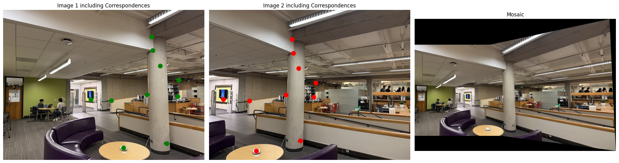
The higher the resulting dot product, the better the match between the two images.</p>

<p>Another option is to use the L2 norm, which can deliver reasonably good results as well. However, the assignment instructions recommended NCC, and I found that it worked well for me.</p>

<h2 id="translation-search-algorithm">Translation Search Algorithm</h2>
<p>Now that we know how to measure a good displacement, how can we actually calculate which displacement is optimal? One idea is to brute-force try all possible translations within a particular range: I used the interval [-15, 15]. 
This algorithm<sup id="fnref:fn-1" role="doc-noteref"><a href="#fn:fn-1" class="footnote" rel="footnote">1</a></sup> is reasonably performant, but it had a problem: it was too slow, taking upwards of 50 seconds for some images. 
We can do better by being smarter about where we search.</p>

<p>Instead of checking every possible displacement, I start with a larger step size to get a rough estimate, and then progressively refine the search with smaller step sizes until I get to pixel-level accuracy. 
This way, we quickly narrow down the promising areas of the search space.</p>

<p>For example, let’s say that we set the max number of search steps to 4: I first try displacements in increments of 4 pixels.
Once I find the best candidate, I reduce the step size to 2 and search in that neighborhood, and finally reduce the step size to 1 to lock in the exact displacement.</p>

<p>Here’s an example of what the algorithm does to a sample image. Notice how neatly aligned the channels are compared to before:</p>
<p align="center">
  <img src="/assets/images/colorize/cathedral_no_pyramid.jpg" width="300" />
</p>

<h1 id="part-2-using-an-image-pyramid">Part 2: Using an Image Pyramid</h1>
<p>The single-scale approach we just discussed works well for lower-resolution JPEG images. But for higher-resolution TIFF images, we need a separate approach: the optimal displacement might be a lot more than 15 pixels in any direction. 
This is where the image pyramid comes in. Here’s how the image pyramid approach works:</p>

<ul>
  <li>Build a pyramid for each channel by repeatedly downsampling by 2 for several levels. I found that having 5 levels worked well for me.</li>
  <li>Start at the coarsest level and align red/green to blue.</li>
  <li>Propagate the found displacement to the next level, scaling by 2. We scale by two because the new image has twice the resolution in both dimensions.</li>
  <li>Refine our estimation at the new level using the single-scale approach described earlier.</li>
  <li>Repeat until you reach the original resolution.</li>
</ul>

<p>This drastically improves results for some images. For example, the Emir of Bukhara image below:</p>

<p>Without the pyramid, it looks like this:</p>
<p align="center">
  <img src="/assets/images/colorize/emir_no_pyramid.jpg" width="450" />
</p>

<p>Conversely, with the pyramid it looks much better:</p>
<p align="center">
  <img src="/assets/images/colorize/emir_pyramid.jpg" width="450" />
</p>

<p>Getting the Emir of Bukhara image to align properly was a big challenge. 
I had to patiently tweak the pyramid levels and search range to get it right.
Even then, my result isn’t perfect because the red channel’s brightness values are very different from those of the blue and green images. 
I think there is a limit to how good the reconstruction can be using just NCC and (x, y) translations.
A more advanced technique like edge detection might be helpful here.</p>

<h1 id="misc-implementation-details">Misc. Implementation Details</h1>
<ul>
  <li>I crop 12.5% off the borders of the image before computing the NCC, as we don’t want border artifacts to influence the final alignment.</li>
  <li>As a post-processing step, I crop 10% off the borders of the final images; the borders of the image contain artifacts from color alignment and are not visually appealing.</li>
  <li>Resizing of images is done via <code class="language-plaintext highlighter-rouge">cv2.resize</code> as opposed to manually applying a Gaussian filter.</li>
</ul>

<h1 id="gallery-of-pyramid-results">Gallery of Pyramid Results</h1>

<p>Here are some of the best results I obtained using the image pyramid approach.
My displacements are in the form (dx, dy).</p>

<table>
  
  
    <tr>
      <td style="text-align:center; padding: 10px; vertical-align: top;">
        <img src="/assets/images/colorize/cathedral_pyramid.jpg" width="400" style="margin: 0 auto; display: block;" /><br />
        <div class="caption">
          cathedral <br />
          Green channel offset: (2, 5) <br />
          Red channel offset: (3, 12)
        </div>
      </td>
    </tr>
  
    <tr>
      <td style="text-align:center; padding: 10px; vertical-align: top;">
        <img src="/assets/images/colorize/church_pyramid.jpg" width="400" style="margin: 0 auto; display: block;" /><br />
        <div class="caption">
          church <br />
          Green channel offset: (4, 25) <br />
          Red channel offset: (-4, 58)
        </div>
      </td>
    </tr>
  
    <tr>
      <td style="text-align:center; padding: 10px; vertical-align: top;">
        <img src="/assets/images/colorize/emir_pyramid.jpg" width="400" style="margin: 0 auto; display: block;" /><br />
        <div class="caption">
          emir <br />
          Green channel offset: (24, 49) <br />
          Red channel offset: (57, 103)
        </div>
      </td>
    </tr>
  
    <tr>
      <td style="text-align:center; padding: 10px; vertical-align: top;">
        <img src="/assets/images/colorize/harvesters_pyramid.jpg" width="400" style="margin: 0 auto; display: block;" /><br />
        <div class="caption">
          harvesters <br />
          Green channel offset: (17, 60) <br />
          Red channel offset: (14, 124)
        </div>
      </td>
    </tr>
  
    <tr>
      <td style="text-align:center; padding: 10px; vertical-align: top;">
        <img src="/assets/images/colorize/icon_pyramid.jpg" width="400" style="margin: 0 auto; display: block;" /><br />
        <div class="caption">
          icon <br />
          Green channel offset: (17, 41) <br />
          Red channel offset: (23, 89)
        </div>
      </td>
    </tr>
  
    <tr>
      <td style="text-align:center; padding: 10px; vertical-align: top;">
        <img src="/assets/images/colorize/italil_pyramid.jpg" width="400" style="margin: 0 auto; display: block;" /><br />
        <div class="caption">
          italil <br />
          Green channel offset: (21, 38) <br />
          Red channel offset: (35, 77)
        </div>
      </td>
    </tr>
  
    <tr>
      <td style="text-align:center; padding: 10px; vertical-align: top;">
        <img src="/assets/images/colorize/melons_pyramid.jpg" width="400" style="margin: 0 auto; display: block;" /><br />
        <div class="caption">
          melons <br />
          Green channel offset: (10, 81) <br />
          Red channel offset: (13, 178)
        </div>
      </td>
    </tr>
  
    <tr>
      <td style="text-align:center; padding: 10px; vertical-align: top;">
        <img src="/assets/images/colorize/monastery_pyramid.jpg" width="400" style="margin: 0 auto; display: block;" /><br />
        <div class="caption">
          monastery <br />
          Green channel offset: (2, -3) <br />
          Red channel offset: (2, 3)
        </div>
      </td>
    </tr>
  
    <tr>
      <td style="text-align:center; padding: 10px; vertical-align: top;">
        <img src="/assets/images/colorize/self_portrait_pyramid.jpg" width="400" style="margin: 0 auto; display: block;" /><br />
        <div class="caption">
          self_portrait <br />
          Green channel offset: (29, 79) <br />
          Red channel offset: (37, 176)
        </div>
      </td>
    </tr>
  
    <tr>
      <td style="text-align:center; padding: 10px; vertical-align: top;">
        <img src="/assets/images/colorize/siren_pyramid.jpg" width="400" style="margin: 0 auto; display: block;" /><br />
        <div class="caption">
          siren <br />
          Green channel offset: (-6, 49) <br />
          Red channel offset: (-25, 96)
        </div>
      </td>
    </tr>
  
    <tr>
      <td style="text-align:center; padding: 10px; vertical-align: top;">
        <img src="/assets/images/colorize/three_generations_pyramid.jpg" width="400" style="margin: 0 auto; display: block;" /><br />
        <div class="caption">
          three_generations <br />
          Green channel offset: (14, 53) <br />
          Red channel offset: (11, 111)
        </div>
      </td>
    </tr>
  
    <tr>
      <td style="text-align:center; padding: 10px; vertical-align: top;">
        <img src="/assets/images/colorize/tobolsk_pyramid.jpg" width="400" style="margin: 0 auto; display: block;" /><br />
        <div class="caption">
          tobolsk <br />
          Green channel offset: (3, 3) <br />
          Red channel offset: (3, 6)
        </div>
      </td>
    </tr>
  
    <tr>
      <td style="text-align:center; padding: 10px; vertical-align: top;">
        <img src="/assets/images/colorize/lastochikino_pyramid.jpg" width="400" style="margin: 0 auto; display: block;" /><br />
        <div class="caption">
          lastochikino <br />
          Green channel offset: (-2, -3) <br />
          Red channel offset: (-9, 75)
        </div>
      </td>
    </tr>
  
    <tr>
      <td style="text-align:center; padding: 10px; vertical-align: top;">
        <img src="/assets/images/colorize/lugano_pyramid.jpg" width="400" style="margin: 0 auto; display: block;" /><br />
        <div class="caption">
          lugano <br />
          Green channel offset: (-16, 41) <br />
          Red channel offset: (-29, 93)
        </div>
      </td>
    </tr>
  
</table>

<h1 id="gallery-of-additional-images-from-the-prokudin-gorskii-collection">Gallery of Additional Images from the Prokudin-Gorskii Collection</h1>
<p>I selected these additional images from the original collection to test my algorithm:</p>

<table>
  
  
    <tr>
      <td style="text-align:center; padding: 10px; vertical-align: top;">
        <img src="/assets/images/colorize/custom0_pyramid.jpg" width="400" style="margin: 0 auto; display: block;" /><br />
        <div class="caption">
          Green channel offset: (3, 29) <br />
          Red channel offset: (-7, 71)
        </div>
      </td>
    </tr>
  
    <tr>
      <td style="text-align:center; padding: 10px; vertical-align: top;">
        <img src="/assets/images/colorize/custom1_pyramid.jpg" width="400" style="margin: 0 auto; display: block;" /><br />
        <div class="caption">
          Green channel offset: (-12, 39) <br />
          Red channel offset: (-27, 86)
        </div>
      </td>
    </tr>
  
    <tr>
      <td style="text-align:center; padding: 10px; vertical-align: top;">
        <img src="/assets/images/colorize/custom2_pyramid.jpg" width="400" style="margin: 0 auto; display: block;" /><br />
        <div class="caption">
          Green channel offset: (-18, 66) <br />
          Red channel offset: (-34, 146)
        </div>
      </td>
    </tr>
  
</table>

<hr />
<div class="footnotes" role="doc-endnotes">
  <ol>
    <li id="fn:fn-1" role="doc-endnote">
      <p>I don’t reproduce the code for this algorithm in this blog post, as per class policies. <a href="#fnref:fn-1" class="reversefootnote" role="doc-backlink">&#8617;</a></p>
    </li>
  </ol>
</div>]]></content><author><name>Vijay Kethanaboyina</name></author><category term="machine learning" /><category term="school project" /><summary type="html"><![CDATA[Colorizing Images of The Russian Empire for my Computer Vision class]]></summary></entry><entry><title type="html">Training a Flow-Matching Policy via Imitation Learning</title><link href="https://www.vkethana.com/pusht/" rel="alternate" type="text/html" title="Training a Flow-Matching Policy via Imitation Learning" /><published>2025-02-11T00:00:00+00:00</published><updated>2025-02-11T00:00:00+00:00</updated><id>https://www.vkethana.com/pusht</id><content type="html" xml:base="https://www.vkethana.com/pusht/"><![CDATA[<p>In Spring 2026, I am taking CS 185, Deep Reinforcement Learning, at UC Berkeley.
This post covers my implementation for Homework 1.
The task is to train an agent to push a T-shaped object into a specific 2D configuration.
In this assignment, we cover two approaches to implementing the policy: MSE and Flow Matching.</p>

<h2 id="mse-policy">MSE Policy</h2>

<p>The Mean-Squared Error (MSE) policy is a straightforward approach to imitation learning with action chunking. In this setup, the policy \(\pi_\theta(o_t)\) maps the current observation \(o_t\) directly to a sequence of future actions \(A_t = (a_t, a_{t+1}, \dots, a_{t+K-1})\), where \(K\) is the chunk size. We use action chunking (sampling K actions from the policy at once) because it reduces the frequency of policy queries and often leads to smoother trajectories.</p>

<h3 id="architecture">Architecture</h3>

<p>For the MSE policy, I used a Multi-Layer Perceptron (MLP) architecture. 
The model takes the 5-dimensional state as input and outputs a flattened vector of size \(K \times \text{action\_dim}\). (Here, the action dimension is two, corresponding to the agent’s target coordinates.)</p>

<ul>
  <li><strong>Hidden Layers</strong>: 3 layers with 512 units each.</li>
  <li><strong>Activation</strong>: ReLU for hidden layers, no activation for the output layer.</li>
  <li><strong>Input Dimension</strong>: 5 (Push-T state).</li>
  <li><strong>Output Dimension</strong>: \(K \times 2\) (Chunk size \(\times\) 2D actions).</li>
</ul>

<h3 id="loss-function">Loss Function</h3>

<p>The policy is trained by minimizing the L2 distance between the predicted action chunk and the expert’s action chunk:</p>

\[L_{MSE}(\theta) = \frac{1}{B} \sum_{j=1}^{B} \| A_t^{(j)} - \pi_\theta(o_t^{(j)}) \|_2^2\]
<h1 id="flow-matching-policy">Flow Matching Policy</h1>

<p>While the MSE policy is simple, it can struggle with multimodal distributions (where the expert might take multiple different valid paths). Flow matching addresses this by learning to transform a simple noise distribution into the expert’s action distribution.</p>

<h3 id="how-it-works">How it Works</h3>

<p>Flow matching learns a conditional vector field \(v_\theta(o_t, A_{t,\tau}, \tau)\) that “pushes” noise samples toward the data distribution. We define a linear interpolation between a noise sample \(A_{t,0} \sim \mathcal{N}(0, I)\) and the expert action chunk \(A_t\):</p>

\[A_{t,\tau} = \tau A_t + (1 - \tau) A_{t,0}\]

<p>The network is then trained to predict the velocity \((A_t - A_{t,0})\) that moves the interpolated sample toward the target:</p>

\[L_{FM}(\theta) = \frac{1}{B} \sum_{j=1}^{B} \| v_\theta(o_t^{(j)}, A_{t,\tau}^{(j)}, \tau^{(j)}) - (A_t^{(j)} - A_{t,0}^{(j)}) \|_2^2\]

<h3 id="inference">Inference</h3>

<p>At test time, we sample \(A_{t,0} \sim \mathcal{N}(0, I)\) and integrate the learned vector field from \(\tau=0\) to \(\tau=1\) using Euler integration:</p>

\[A_{t,\tau + \Delta\tau} = A_{t,\tau} + \Delta\tau \cdot v_\theta(o_t, A_{t,\tau}, \tau)\]

<p>This iteratively refines the action starting from pure noise. The exact number of denoising steps (which determines the value of $\Delta\tau$) is <strong>30</strong> for my training runs.</p>

<h1 id="results">Results</h1>

<h3 id="mse-policy-results">MSE Policy Results</h3>

<p><strong>Training Curves</strong></p>

<p><img src="/assets/images/pusht/mse_train.jpg" alt="MSE Training Loss" />
<img src="/assets/images/pusht/mse_reward.jpg" alt="MSE Reward" /></p>

<p><strong>Performance Videos</strong></p>

<table>
  <thead>
    <tr>
      <th style="text-align: center">Before Training</th>
      <th style="text-align: center">After Training</th>
    </tr>
  </thead>
  <tbody>
    <tr>
      <td style="text-align: center"><video src="/assets/videos/pusht/mse_start_1.mp4" controls="" width="100%"></video></td>
      <td style="text-align: center"><video src="/assets/videos/pusht/mse_end_1.mp4" controls="" width="100%"></video></td>
    </tr>
  </tbody>
</table>

<h3 id="flow-matching-policy-results">Flow Matching Policy Results</h3>

<p><strong>Training Curves</strong></p>

<p><img src="/assets/images/pusht/fm_train.jpg" alt="Flow Matching Training Loss" />
<img src="/assets/images/pusht/fm_reward.jpg" alt="Flow Matching Reward" /></p>

<p><strong>Performance Videos</strong></p>

<table>
  <thead>
    <tr>
      <th style="text-align: center">Before Training</th>
      <th style="text-align: center">After Training</th>
    </tr>
  </thead>
  <tbody>
    <tr>
      <td style="text-align: center"><video src="/assets/videos/pusht/flow_start_1.mp4" controls="" width="100%"></video></td>
      <td style="text-align: center"><video src="/assets/videos/pusht/flow_end_1.mp4" controls="" width="100%"></video></td>
    </tr>
  </tbody>
</table>

<h2 id="qualitative-comparison">Qualitative Comparison</h2>

<p>Qualitatively, we observe several key differences between the MSE and Flow Matching policies in the Push-T environment:</p>

<ul>
  <li><strong>Initialization and Early Training</strong>: At the start of training, the flow matching policy appears “jittery” and erratic. This is because it is sampling from a noise distribution and the vector field is not yet well-defined. In contrast, the untrained MSE policy tends to output a mean action that often results in the agent staying static or moving in an unhelpful direction.</li>
  <li><strong>Final Performance</strong>: By the end of training, the flow matching policy significantly outperforms the MSE policy. The flow matching agent demonstrates clearer evidence of “planning”. It (re-)orients itself correctly relative to the T-block and makes purposeful pushes toward the goal.</li>
  <li><strong>The “Mean Action” Problem</strong>: The performance gap is likely due to the training objective. An MSE policy learns to predict the average expert action for a given state. In multimodal scenarios (e.g., if an expert sometimes goes left and sometimes goes right to push the block), the MSE policy will predict the average, which may be straight into the block—leading to suboptimal behavior. Flow matching, being a generative model, can represent these multiple modes effectively, allowing it to “commit” to one valid path.</li>
</ul>

<h2 id="conclusion">Conclusion</h2>

<p>This assignment was fun. My next steps are to train policies for harder environments than Push-T, which will naturally necessitate the use of techniques more sophisticated than mere imitation learning. 
More on that coming soon!</p>]]></content><author><name>Vijay Kethanaboyina</name></author><category term="machine learning" /><category term="school project" /><summary type="html"><![CDATA[In Spring 2026, I am taking CS 185, Deep Reinforcement Learning, at UC Berkeley. This post covers my implementation for Homework 1. The task is to train an agent to push a T-shaped object into a specific 2D configuration. In this assignment, we cover two approaches to implementing the policy: MSE and Flow Matching.]]></summary></entry><entry><title type="html">Generating Cognateful Sentences with Large Language Models</title><link href="https://www.vkethana.com/cognateful/" rel="alternate" type="text/html" title="Generating Cognateful Sentences with Large Language Models" /><published>2025-01-05T00:00:00+00:00</published><updated>2025-01-05T00:00:00+00:00</updated><id>https://www.vkethana.com/cognateful</id><content type="html" xml:base="https://www.vkethana.com/cognateful/"><![CDATA[<h1 id="motivation">Motivation</h1>
<blockquote>
  <p>“Le président Emmanuel Macron assure le peuple canadien que le gouvernement français va continuer à défendre le Canada contre la menace américain.”</p>
</blockquote>

<p>Even if you don’t speak French, you can probably understand, or at least get the gist of, the above sentence: the French president Emmanuel Macron is assuring the “peuple canadien” (Canadian people) about something involving the “gouvernment français” (French government). 
Imagine reading thousands of sentences like this and gradually acquiring French through cognates you already know. 
This is a type of comprehensible input, a language learning technique popularized by linguist Stephen Krashen in the 1980s.</p>

<p>Comprehensible input is a good language learning method, but creating it is very hard. 
A native speaker has to painstakingly create thousands of sentences that speakers of another language can understand, gradually increasing the difficulty as the learner progresses. 
Resources like this actually do exist for a number of languages. 
For example, learners of Latin can use <em>Lingua Latina per se Illustrata</em>, a book that teaches you Latin using exclusively sentences in Latin. 
However, writing this text took years of effort on the part of Hans Ørberg, a linguist who dedicated a large part of his life to teaching Latin.
Ørberg carefully wrote the sentences in his book to only use cognates an English speaker could understand and to avoid any complicated syntax an English speaker would have a hard time understanding.</p>

<p>What if there was a way to automate the process of generating “cognateful” sentences using large language models? 
Language models like GPT-4o and o1 have good enough reasoning ability to tell what words in a foreign language are and aren’t cognate with English. 
They can reliably generate sentences in other languages like French without any additional training.
In short, this is an ideal use case for LLMs.</p>

<h1 id="what-i-did">What I did</h1>
<p>I made a simple interactive language-learning app, hosted at <a href="https://cognateful.vkethana.com">cognateful.vkethana.com</a>. It teaches you French using stories written exclusively in French.</p>

<p>Users are provided with a brief, ten-sentence story consisting of French sentences. The user’s task is to read the sentences and translate them into English. 
The app tells you whether or not your translation is correct using GPT-4o-powered scoring. 
Based on your performance on the exercises, it assigns you a “difficulty” score, which goes up and down depending on your performance. 
Users then are served sentences at appropriate levels of difficulty based on their performance. For those who are curious, the source code for this project can be found <a href="https://github.com/vkethana/cognate_sentences">here</a>.</p>

<p>Caveats: This is just a minimum viable product. 
The number of sentences in the app is limited. 
I don’t speak French (yet), so sentences may contain mistakes.
But the interface, scoring system, and sentence generation are all functional, and I think they will work at scale. 
The biggest hurdle to improving the app is increasing the number of sentences while not compromising on sentence quality.</p>

<h1 id="how-i-generated-and-scored-the-sentences">How I generated and scored the sentences</h1>
<h2 id="scoring">Scoring</h2>
<p>I have to explain sentence scoring before sentence generation because the scoring system influenced the prompt used to generate the sentences. 
I give o1-preview a sentence and ask it to score its difficulty on a scale of 0 to 3, 0 being very hard to understand for a monolingual English speaker and 3 being very easy.</p>

<p><strong>Score 0</strong>: Completely unintelligible to English speakers.
Example: “Je veux manger du pain.”</p>

<p><strong>Score 1</strong>: Contains some cognate words, but contains words unintelligible to an English speaker. The cognates might allow them to guess the general topic but not the main idea or actual meaning. Example: “Le maître savant utilise beaucoup de livres.” (Has cognates like “savant” but key verbs/objects aren't cognates)</p>

<p><strong>Score 2:</strong> Contains many cognate words. An English speaker might guess the main idea but would miss important details or nuances that change the meaning. Example: “Le patient refuse absolument de prendre ses médicaments malgré les protestations constantes du docteur.” <sup id="fnref:fn-1" role="doc-noteref"><a href="#fn:fn-1" class="footnote" rel="footnote">1</a></sup></p>

<p><strong>Score 3:</strong> Fully understandable through cognates. Use almost exclusively cognate words except for basic connectors. Example: “Le président Emmanuel Macron assure le peuple canadien que le gouvernement français va continuer à défendre le Canada contre la menace américain.”</p>

<p>(Side Note: I found that using o1-preview is necessary for good-quality scoring. 
Other models – 4o, 4o-mini, and o1-mini – had a hard time determining what a cognate was. 
Also, they were too lenient, often assigning scores of 3 to sentences that in my opinion an English speaker wouldn’t be able to fully understand.
Even o1-preview sometimes uses words an English speaker wouldn’t understand.)</p>

<h2 id="generation">Generation</h2>
<p>To save time and money, I pregenerate all sentences on the site using GPT-4o and o1-preview. 
Unsurprisingly, o1 made much higher quality sentences, but 4o did a pretty good job too, and any bad-quality sentences are flagged by the scoring system anyway. So it’s OK to cut costs and use a cheaper model when generating sentences, but not when scoring them.
To generate sentences, I made a function <code class="language-plaintext highlighter-rouge">generate_story</code> that takes in a target difficulty and then asks GPT-4o to generate a story consisting of sentences at that difficulty. This allows me to create a variety of sentences at different difficulty levels to suit the user’s needs.</p>

<p>To make the final set of sentences seen on the site, my script repeatedly calls, and saves the output of, <code class="language-plaintext highlighter-rouge">generate_story</code> with the target difficulty set to a randomly-generated integer between 0 and 3, inclusive. 
Here’s a breakdown of how many sentences the site currently has per difficulty level (recall that 1 story = 10 sentences).</p>

<table>
  <thead>
    <tr>
      <th>Score Range</th>
      <th># Sentences Available</th>
    </tr>
  </thead>
  <tbody>
    <tr>
      <td>0.00-0.99</td>
      <td>30</td>
    </tr>
    <tr>
      <td>1.00-1.99</td>
      <td>110</td>
    </tr>
    <tr>
      <td>2.00-2.49</td>
      <td>120</td>
    </tr>
    <tr>
      <td>2.50-3.00</td>
      <td>190</td>
    </tr>
  </tbody>
</table>

<details>
<summary>
For those interested, the exact prompts used to score and generate sentences are below (click me!):
</summary>
<div>
    <div class="language-python highlighter-rouge"><div class="highlight"><pre class="highlight"><code><span class="c1"># Source code: https://github.com/vkethana/cognate_sentences
</span><span class="n">client</span> <span class="o">=</span> <span class="n">OpenAI</span><span class="p">(</span><span class="n">api_key</span><span class="o">=</span><span class="n">os</span><span class="p">.</span><span class="n">environ</span><span class="p">[</span><span class="s">"OPENAI_API_KEY"</span><span class="p">])</span>
<span class="n">language_codes</span> <span class="o">=</span> <span class="p">{</span>
    <span class="s">'fr'</span><span class="p">:</span> <span class="s">'French'</span>
<span class="p">}</span>
<span class="n">SENTENCE_GENERATION_MODEL</span> <span class="o">=</span> <span class="s">'gpt-4o'</span>
<span class="n">SENTENCE_SCORING_MODEL</span> <span class="o">=</span> <span class="s">'o1-preview'</span> <span class="c1"># 'o1' doesn't work for some reason
</span> 
<span class="k">def</span> <span class="nf">generate_story</span><span class="p">(</span><span class="n">lang_code</span><span class="p">,</span> <span class="n">num_sentences</span><span class="p">,</span> <span class="n">target_difficulty</span><span class="p">):</span>
    <span class="n">system_prompt</span> <span class="o">=</span> <span class="sa">f</span><span class="s">"""
    You are a fluent speaker of both </span><span class="si">{</span><span class="n">language_codes</span><span class="p">[</span><span class="n">lang_code</span><span class="p">]</span><span class="si">}</span><span class="s"> and English.
    Generate exactly </span><span class="si">{</span><span class="n">num_sentences</span><span class="si">}</span><span class="s"> </span><span class="si">{</span><span class="n">language_codes</span><span class="p">[</span><span class="n">lang_code</span><span class="p">]</span><span class="si">}</span><span class="s"> sentences that:
    1. Form a coherent narrative where each sentence follows from the previous one
    2. Target difficulty level </span><span class="si">{</span><span class="n">target_difficulty</span><span class="si">}</span><span class="s"> using these criteria:

        Level 0: Completely unintelligible to English speakers.
        Example: "Je veux manger du pain."

        Level 1: Contains some cognate words, but is largely unintelligible to an English speaker. The cognates might allow them to guess the general topic but not the actual meaning.
        Example: "Le maître savant utilise beaucoup de livres." (Has cognates like "savant" but key verbs/objects aren</span><span class="se">\'</span><span class="s">t cognates)

        Level 2: Contains many cognate words. An English speaker could understand the main idea but would miss important details or nuances that change the meaning.
        Example: "Le patient refuse absolument de prendre ses médicaments malgré les protestations constantes du docteur."
        An English speaker would get "patient refuses absolutely to take medications" and "constant protestations doctor" but might miss "his" and "despite", changing their understanding of whose medications and the relationship between the refusal and protestations.

        Level 3: Fully understandable through cognates. Use almost exclusively cognate words except for basic connectors.
        Example: "Le président Emmanuel Macron assure le peuple canadien que le gouvernement français va continuer à défendre le Canada contre la menace américain."

        DIFFICULTY TARGETING STRATEGIES:
        Difficulty 0: Use basic, high-frequency native vocabulary, avoid international words
        Difficulty 1: Use 25-30% cognates in non-crucial positions. Has cognates but leaves major meaning gaps.
        Difficulty 2: Use 50-60% cognates in main concept positions. Sentence is mostly understandable but has subtle meaning changes due to missed words</span><span class="se">\n</span><span class="s">
        Difficulty 3: Use 80-90% cognates, especially for key meaning-bearing words. Any small connecting words (le, que, etc.) can be ignored without losing meaning. Should be assigned sparingly - only when missed words don</span><span class="se">\'</span><span class="s">t change meaning</span><span class="se">\n</span><span class="s">

    Format your response as a JSON array of </span><span class="si">{</span><span class="n">num_sentences</span><span class="si">}</span><span class="s"> objects:
    {{
        "sentence": "&lt;Generated sentence&gt;",
        "target_difficulty": </span><span class="si">{</span><span class="n">target_difficulty</span><span class="si">}</span><span class="s">,
        "reasoning": "&lt;Why this sentence matches difficulty. If this is not the first sentence, also explain why this continues the story from the previous sentence in this JSON array.&gt;",
        "cognate_words": [&lt;List of cognates used&gt;]
    }}

    Important: Each sentence must directly follow from the previous one to form a coherent story.
    Generate </span><span class="si">{</span><span class="n">num_sentences</span><span class="si">}</span><span class="s"> sentences meeting these criteria (difficulty level and story continuation).
    Note: Please do not include Markdown formatting tags (```) in your response, as my parser will not be able to interpret them.
    """</span>
    
    <span class="n">response</span> <span class="o">=</span> <span class="n">client</span><span class="p">.</span><span class="n">chat</span><span class="p">.</span><span class="n">completions</span><span class="p">.</span><span class="n">create</span><span class="p">(</span>
        <span class="n">model</span><span class="o">=</span><span class="n">SENTENCE_GENERATION_MODEL</span><span class="p">,</span>
        <span class="n">messages</span><span class="o">=</span><span class="p">[{</span><span class="s">'role'</span><span class="p">:</span> <span class="s">'user'</span><span class="p">,</span> <span class="s">'content'</span><span class="p">:</span> <span class="n">system_prompt</span><span class="p">}],</span>
        <span class="n">temperature</span><span class="o">=</span><span class="mf">1.0</span>
    <span class="p">)</span>
    
    <span class="c1"># Parse generated sentences
</span>    <span class="k">return</span> <span class="n">json</span><span class="p">.</span><span class="n">loads</span><span class="p">(</span><span class="n">response</span><span class="p">.</span><span class="n">choices</span><span class="p">[</span><span class="mi">0</span><span class="p">].</span><span class="n">message</span><span class="p">.</span><span class="n">content</span><span class="p">)</span>

<span class="k">def</span> <span class="nf">gpt_scored_rubric_batch</span><span class="p">(</span><span class="n">sentences</span><span class="p">):</span>
    <span class="s">'''
    Score multiple French sentences at once using GPT-4.

    Args:
        sentences: List of sentences to score
    Returns:
        List of scoring results
    '''</span>

    <span class="n">system_prompt</span> <span class="o">=</span> <span class="sa">f</span><span class="s">"""
    You are an expert in French to English translation. I will give you </span><span class="si">{</span><span class="nb">len</span><span class="p">(</span><span class="n">sentences</span><span class="p">)</span><span class="si">}</span><span class="s"> sentences in French, and I want you to score each of them on a scale from 0-3 using the following rubric:

    0: Completely unintelligible to English speakers.
    Example: "Je veux manger du pain."

    1: Contains some cognate words, but contains words unintelligible to an English speaker. The cognates might allow them to guess the general topic but not the main idea or actual meaning.
    Example: "Le maître savant utilise beaucoup de livres." (Has cognates like "savant" but key verbs/objects aren</span><span class="se">\'</span><span class="s">t cognates)

    2: Contains many cognate words. An English speaker might guess the main idea but would miss important details or nuances that change the meaning.
    Example: "Le patient refuse absolument de prendre ses médicaments malgré les protestations constantes du docteur."
    An English speaker would get "patient refuses absolutely to take medications" and "constant protestations doctor" but might miss "his" and "despite", changing their understanding of whose medications and the relationship between the refusal and protestations.

    3: Fully understandable through cognates. Use almost exclusively cognate words except for basic connectors.
    Example: "Le président Emmanuel Macron assure le peuple canadien que le gouvernement français va continuer à défendre le Canada contre la menace américain."

    Important scoring notes:
    - Score 0 sentences have little to no cognates
    - Score 1 sentences have cognates but leave major meaning gaps
    - Score 2 sentences are mostly understandable but have subtle meaning changes due to missed words
    - Score 3 should be assigned sparingly - only when missed words don’t change meaning

    For each sentence, provide a JSON object with these fields:
    {{
      "sentence": "&lt;Sentence&gt;",
      "cognate_words": [&lt;List of Cognate Words&gt;],
      "reasoning": "&lt;Reasoning for the score&gt;",
      "score": &lt;Numerical for the Sentence (0-3)&gt;
    }} 

    Please format your response as a JSON array of these objects. You should have </span><span class="si">{</span><span class="nb">len</span><span class="p">(</span><span class="n">sentences</span><span class="p">)</span><span class="si">}</span><span class="s"> objects in your array.

    Here are the sentences to score:
    </span><span class="si">{</span><span class="n">json</span><span class="p">.</span><span class="n">dumps</span><span class="p">(</span><span class="n">sentences</span><span class="p">,</span> <span class="n">ensure_ascii</span><span class="o">=</span><span class="bp">False</span><span class="p">)</span><span class="si">}</span><span class="s">
    Note: Please do not include Markdown formatting tags (```) in your response, as my parser will not be able to interpret them.
    """</span>

    <span class="n">completion</span> <span class="o">=</span> <span class="n">client</span><span class="p">.</span><span class="n">chat</span><span class="p">.</span><span class="n">completions</span><span class="p">.</span><span class="n">create</span><span class="p">(</span>
        <span class="n">model</span><span class="o">=</span><span class="n">SENTENCE_SCORING_MODEL</span><span class="p">,</span>
        <span class="n">messages</span><span class="o">=</span><span class="p">[</span>
            <span class="p">{</span><span class="s">'role'</span><span class="p">:</span> <span class="s">'user'</span><span class="p">,</span> <span class="s">'content'</span><span class="p">:</span> <span class="n">system_prompt</span><span class="p">}</span>
        <span class="p">],</span>
        <span class="n">temperature</span><span class="o">=</span><span class="mi">1</span>
    <span class="p">)</span>
    
    <span class="n">response_text</span> <span class="o">=</span> <span class="n">completion</span><span class="p">.</span><span class="n">choices</span><span class="p">[</span><span class="mi">0</span><span class="p">].</span><span class="n">message</span><span class="p">.</span><span class="n">content</span><span class="p">.</span><span class="n">strip</span><span class="p">()</span>
    <span class="k">try</span><span class="p">:</span>
        <span class="n">results</span> <span class="o">=</span> <span class="n">json</span><span class="p">.</span><span class="n">loads</span><span class="p">(</span><span class="n">response_text</span><span class="p">)</span>
        <span class="k">return</span> <span class="n">results</span>
    <span class="k">except</span> <span class="n">json</span><span class="p">.</span><span class="n">JSONDecodeError</span><span class="p">:</span>
        <span class="k">print</span><span class="p">(</span><span class="s">"Error: Failed to decode JSON from the response."</span><span class="p">)</span>
        <span class="k">raise</span>
</code></pre></div>    </div>
  </div>
</details>
<h1 id="approaches-that-didnt-work">Approaches that didn’t work</h1>
<ul>
  <li><strong>Sentence starters:</strong> 
I was initially worried that repeatedly asking the model to generate sentences would result in the same stories being generated over and over. 
To deal with this, I modified my prompt to randomly pick a sentence starter from a hardcoded list of unfinished French sentences. I then asked the model to generate sentences which continued off the sentence starter.
This works, but I eventually got rid of it and found that the sentences were still diverse enough.</li>
  <li><strong>Live generation:</strong>
Rather than pre-generating the sentences, I originally thought about generating them on the spot and feeding the model with information about the user’s past performance.
But pre-generating sentences is cheaper, and we can still adapt to the user’s performance using the scoring system.</li>
  <li><strong>Cognate ratios:</strong>
Originally, I scored sentences using a weighted combination of GPT-4’s judgments and the percentage of cognate words in the sentence. 
This is a bad idea because it treats all cognate words equally, leading to inaccurate scoring. 
For example, “ouvre” and “technologie” are both cognates, but the latter is much easier to understand.
A possible fix for this problem is to take into account the age of acquisition (AoA) of the cognate words.
I plan to return to this idea, using a system that gives better scores to some cognate words.</li>
</ul>

<h1 id="some-optimizations-i-made">Some optimizations I made</h1>
<ul>
  <li><strong>Chain of Thought Prompting</strong>: I tell the model to reason through its scoring and generation process. This substantially reduces hallucinations and improves the output quality of weaker models.
For example, my prompt for sentence scoring tells the LM to use the following output in its response:</li>
</ul>

<div class="language-json highlighter-rouge"><div class="highlight"><pre class="highlight"><code><span class="w">    </span><span class="p">{</span><span class="w">
      </span><span class="nl">"sentence"</span><span class="p">:</span><span class="w"> </span><span class="s2">"&lt;Sentence&gt;"</span><span class="p">,</span><span class="w">
      </span><span class="nl">"cognate_words"</span><span class="p">:</span><span class="w"> </span><span class="s2">"[&lt;List of Cognate Words&gt;]"</span><span class="p">,</span><span class="w">
      </span><span class="nl">"reasoning"</span><span class="p">:</span><span class="w"> </span><span class="s2">"&lt;Reasoning for the score&gt;"</span><span class="p">,</span><span class="w">
      </span><span class="nl">"score"</span><span class="p">:</span><span class="w"> </span><span class="s2">"&lt;Numerical for the Sentence (0-3)&gt;"</span><span class="w">
    </span><span class="p">}</span><span class="w">
</span></code></pre></div></div>
<ul>
  <li><strong>Batching LLM calls to reduce inference costs:</strong> Sentences are generated and scored in batches of 10, which brings down the cost and time of generating and scoring stories a lot.</li>
  <li><strong>Require JSON outputs:</strong> I wasted a lot of time trying to get the LM to output in a format that was easy to parse in Python. Eventually I realized that JSON outputs were perfect for this situation. 
Anecdotally, it feels like formatting-related hallucinations are less common when the model is tasked with outputting JSON and not an ad-hoc, user-defined format.</li>
</ul>

<h1 id="findings">Findings</h1>
<p>With the right prompting and search strategy, LLMs can definitely generate “cognateful” sentences. I think all three of these examples can be mostly understood by an English speaker:</p>

<blockquote>
  <p>Netflix est une plateforme de streaming vidéo qui offre une large sélection de films, séries télévisées et documentaires.</p>
</blockquote>

<blockquote>
  <p>L’intellectuel français Voltaire a dit: “La tolérance est un ingrédient essentiel de la civilisation.”</p>
</blockquote>

<blockquote>
  <p>En 1310, le navigateur italien Marco Polo a traversé l’océan Indien.</p>
</blockquote>

<p>Some cognate words have a stronger association with high-scoring sentences than others. 
For example, <em>université</em> and <em>enthousiasme</em> have average scores of 3.00, whereas <em>recherches</em> and <em>ouvre</em> have average scores of 1.67. 
These findings might seem obvious at first glance, but it’s proof that the scoring function is doing something right!
Cognates that are very easy to understand receive high scores. 
More difficult or obscure cognates receive lower scores.
Here’s a non-exhaustive table of some cognates and the average scores of the sentences containing them.</p>

<table>
  <thead>
    <tr>
      <th>1.00 - 1.99</th>
      <th>2.00 - 2.99</th>
      <th>3.00</th>
    </tr>
  </thead>
  <tbody>
    <tr>
      <td>arbre</td>
      <td>internationale</td>
      <td>université</td>
    </tr>
    <tr>
      <td>mystérieux</td>
      <td>succès</td>
      <td>applaudissent</td>
    </tr>
    <tr>
      <td>Après</td>
      <td>célèbre</td>
      <td>admire</td>
    </tr>
    <tr>
      <td>impatience</td>
      <td>présente</td>
      <td>directeur</td>
    </tr>
    <tr>
      <td>forêt</td>
      <td>entier</td>
      <td>exposition</td>
    </tr>
    <tr>
      <td>ensemble</td>
      <td>Paris</td>
      <td>annonce</td>
    </tr>
    <tr>
      <td>ouvre</td>
      <td>musée</td>
      <td>communauté</td>
    </tr>
    <tr>
      <td>contribution</td>
      <td>musicien</td>
      <td>invitation</td>
    </tr>
    <tr>
      <td>recherches</td>
      <td>moderne</td>
      <td>accepte</td>
    </tr>
    <tr>
      <td>chat</td>
      <td>nouvelle</td>
      <td>enthousiasme</td>
    </tr>
    <tr>
      <td>Thomas</td>
      <td>organise</td>
      <td>révolutionnaire</td>
    </tr>
    <tr>
      <td>cuisine</td>
      <td>principal</td>
      <td>invite</td>
    </tr>
    <tr>
      <td>porte</td>
      <td>problème</td>
      <td>technologie</td>
    </tr>
    <tr>
      <td>lit</td>
      <td>académique</td>
      <td>immédiatement</td>
    </tr>
    <tr>
      <td>Luc</td>
      <td>économique</td>
      <td>planifier</td>
    </tr>
    <tr>
      <td>soleil</td>
      <td>voyager</td>
      <td>collection</td>
    </tr>
    <tr>
      <td>mais</td>
      <td>secret</td>
      <td>objet</td>
    </tr>
    <tr>
      <td>entre</td>
      <td>performance</td>
      <td>éducation</td>
    </tr>
    <tr>
      <td>livre</td>
      <td>formule</td>
      <td>thème</td>
    </tr>
    <tr>
      <td>cherche</td>
      <td>incroyable</td>
      <td> </td>
    </tr>
    <tr>
      <td> </td>
      <td>monde</td>
      <td> </td>
    </tr>
    <tr>
      <td> </td>
      <td>professeur</td>
      <td> </td>
    </tr>
    <tr>
      <td> </td>
      <td>conférence</td>
      <td> </td>
    </tr>
  </tbody>
</table>

<details>
<summary>
Click to see the raw data used to make the above table
</summary>
<div>
    <p>Note that the list only contains words which appear at least two times across all the sentences. Also, the table above isn’t exhaustive.</p>
    <div class="language-plaintext highlighter-rouge"><div class="highlight"><pre class="highlight"><code>Cognate Words Sorted by Average Score:
université: 3.00
importante: 3.00
spectateurs: 3.00
applaudissent: 3.00
découverte: 3.00
dans: 3.00
urgente: 3.00
révèle: 3.00
admire: 3.00
sculptures: 3.00
équipe: 3.00
directeur: 3.00
technique: 3.00
exposition: 3.00
inclut: 3.00
beaucoup: 3.00
annonce: 3.00
étudiant: 3.00
présenter: 3.00
communauté: 3.00
anciennes: 3.00
invitation: 3.00
accepte: 3.00
enthousiasme: 3.00
applaudit: 3.00
renommée: 3.00
Le: 3.00
révolutionnaire: 3.00
la: 3.00
invite: 3.00
technologie: 3.00
immédiatement: 3.00
globales: 3.00
planifier: 3.00
vaisseau: 3.00
spatial: 3.00
atteint: 3.00
contacte: 3.00
agent: 3.00
crée: 3.00
reconnaissance: 3.00
collection: 3.00
acclamation: 3.00
encouragé: 3.00
peintures: 3.00
modernes: 3.00
objet: 3.00
propre: 3.00
exposer: 3.00
idée: 3.00
potentiel: 3.00
énorme: 3.00
vision: 3.00
nationale: 3.00
éducation: 3.00
système: 3.00
théories: 3.00
gagne: 3.00
talent: 3.00
acceptent: 3.00
énergie: 3.00
artistique: 3.00
peut: 3.00
ville: 3.00
Daniel: 3.00
physique: 3.00
Leur: 3.00
thème: 3.00
Londres: 3.00
Marie: 3.00
hôtel: 3.00
glaciers: 3.00
internationale: 2.93
succès: 2.90
célèbre: 2.87
présente: 2.83
entier: 2.83
Paris: 2.82
musée: 2.80
musicien: 2.80
moderne: 2.80
nouvelle: 2.79
organise: 2.78
principal: 2.75
problème: 2.75
académique: 2.75
économique: 2.75
voyager: 2.75
secret: 2.75
performance: 2.75
formule: 2.75
Les: 2.75
incroyable: 2.75
monde: 2.73
professeur: 2.72
conférence: 2.72
situation: 2.71
propose: 2.71
reçoit: 2.71
innovante: 2.67
amis: 2.67
étranger: 2.67
marche: 2.67
grande: 2.67
inspiration: 2.67
plan: 2.67
action: 2.67
ambitieux: 2.67
planète: 2.67
diffusent: 2.67
explorer: 2.67
avancée: 2.67
internationales: 2.67
prestigieux: 2.67
document: 2.67
résultats: 2.67
réalise: 2.67
autorités: 2.67
visiter: 2.67
positive: 2.67
œuvre: 2.67
discutent: 2.67
collaborer: 2.67
arrivent: 2.67
diplomates: 2.67
inspire: 2.60
découvrent: 2.60
finalement: 2.60
spectaculaire: 2.60
projet: 2.60
attention: 2.60
article: 2.60
artiste: 2.59
événement: 2.57
médias: 2.57
mission: 2.57
Finalement: 2.57
scientifique: 2.53
étudiants: 2.50
extraordinaire: 2.50
apparaît: 2.50
solution: 2.50
décide: 2.50
habitants: 2.50
réunion: 2.50
ancienne: 2.50
documents: 2.50
président: 2.50
gouvernement: 2.50
détails: 2.50
experts: 2.50
impact: 2.50
solutions: 2.50
Europe: 2.50
décident: 2.50
concert: 2.50
traditionnelle: 2.50
information: 2.50
gouvernements: 2.50
astronautes: 2.50
commencent: 2.50
spatiale: 2.50
animaux: 2.50
exotiques: 2.50
entrée: 2.50
grotte: 2.50
inscriptions: 2.50
hésite: 2.50
dangereuse: 2.50
fans: 2.50
soir: 2.50
admiration: 2.50
David: 2.50
palais: 2.50
innovation: 2.50
prix: 2.50
exceptionnelles: 2.50
excitation: 2.50
collaborent: 2.50
ingénieurs: 2.50
refuge: 2.50
important: 2.50
national: 2.50
menace: 2.50
nation: 2.50
étudier: 2.50
retourne: 2.50
réalité: 2.50
Avec: 2.50
scène: 2.50
style: 2.50
tableau: 2.50
unique: 2.50
New York: 2.50
histoire: 2.50
développement: 2.50
collègues: 2.50
presse: 2.50
locales: 2.50
universités: 2.50
visiteurs: 2.50
organiser: 2.50
mondiale: 2.50
intelligence: 2.50
interrompt: 2.50
recherche: 2.50
inspiré: 2.50
attire: 2.50
international: 2.50
discuter: 2.50
climatique: 2.50
œuvres: 2.50
nouveau: 2.50
complexes: 2.50
film: 2.50
mer: 2.50
participer: 2.50
démonstration: 2.50
très: 2.50
réunions: 2.50
Lucie: 2.50
voyage: 2.46
est: 2.45
commence: 2.43
art: 2.43
découvre: 2.40
public: 2.40
musique: 2.40
peinture: 2.40
incident: 2.33
docteur: 2.33
magnifiques: 2.33
continue: 2.33
nouvelles: 2.33
aventure: 2.33
explorent: 2.33
célèbres: 2.33
extraterrestre: 2.33
change: 2.33
humanité: 2.33
expédition: 2.33
rencontre: 2.33
Pierre: 2.33
internationaux: 2.33
curieux: 2.33
intérêt: 2.33
critique: 2.33
révélation: 2.33
exprime: 2.33
rapidement: 2.30
initiative: 2.25
nombreux: 2.25
grand: 2.25
participants: 2.25
galerie: 2.22
offre: 2.20
scientifiques: 2.20
arrive: 2.17
visite: 2.17
mystérieuse: 2.14
présentation: 2.00
brillante: 2.00
village: 2.00
enfants: 2.00
avec: 2.00
alarme: 2.00
affirme: 2.00
citoyens: 2.00
mesures: 2.00
résoudre: 2.00
critiques: 2.00
changements: 2.00
prépare: 2.00
historiques: 2.00
souvenirs: 2.00
observe: 2.00
groupe: 2.00
lettre: 2.00
étrange: 2.00
soupe: 2.00
plats: 2.00
France: 2.00
pour: 2.00
cabane: 2.00
analysent: 2.00
informations: 2.00
incroyables: 2.00
idées: 2.00
espion: 2.00
aide: 2.00
couvre: 2.00
encore: 2.00
certains: 2.00
innovantes: 2.00
conférences: 2.00
invité: 2.00
magnifique: 2.00
française: 2.00
Isabelle: 2.00
acteurs: 2.00
paysage: 2.00
jour: 2.00
significative: 2.00
mystérieux: 1.83
Après: 1.80
impatience: 1.75
forêt: 1.67
ensemble: 1.67
ouvre: 1.67
contribution: 1.67
recherches: 1.67
chat: 1.67
Thomas: 1.67
cuisine: 1.60
ami: 1.50
trésor: 1.50
secrète: 1.50
femme: 1.50
table: 1.50
monte: 1.50
le: 1.50
étranges: 1.50
porte: 1.50
lit: 1.50
sombre: 1.50
projets: 1.50
suit: 1.50
support: 1.50
professeurs: 1.50
long: 1.50
Luc: 1.40
soleil: 1.33
mais: 1.33
entre: 1.33
livre: 1.33
cherche: 1.25
maison: 1.00
famille: 1.00
part: 1.00
arbre: 1.00
et: 1.00
matin: 1.00
</code></pre></div>    </div>
  </div>
</details>
<h1 id="features-i-plan-to-add">Features I plan to add</h1>
<ul>
  <li>Scale up the number of sentences in the app.</li>
  <li>Bring back beam search for sentence generation: Currently I’m making stories by generating 10 sentences at once. A better, but slower and more costly, way to get high-scoring sentences is to generate many options, expand the highest-scoring ones, and discard the rest, gradually building up the stories.</li>
  <li>Remove all English from the UI. Instead, express UI functions using images and icons. Any words which appear on the screen should be in the target language, not English, in order to immerse the user as much as possible.</li>
  <li>Come up with better heuristics for bumping up and down the user’s difficulty score based on their performance. Right now, we simply decrement / increment the user’s difficulty by 0.10 for each correct or incorrect answer. (Note that lower difficulty values = harder, not easier, sentences)</li>
  <li><strong>Improve sentence scoring:</strong> I think that this is the hardest part of the project and that the sentence scoring has a lot of room for improvement. 
For example, I could modify the scoring system to use a weighted combination<sup id="fnref:fn-2" role="doc-noteref"><a href="#fn:fn-2" class="footnote" rel="footnote">2</a></sup> of two things: GPT-4 judgement scoring and the presence of certain high-scoring cognate words (see “Findings” above).</li>
  <li>Add support for languages other than English.</li>
</ul>

<h1 id="how-you-can-help">How you can help</h1>
<p>If you’re familiar with NLP, linguistics, or software development, you can help out by suggesting solutions to the following blockers that I’m currently facing.</p>
<ul>
  <li><strong>Cheaper and faster scoring</strong>:
Is there a cheaper, more scalable way to score sentences than what I’ve described here?
To recap, using reasoning models like o1 is effective but slow and expensive.
Using models other than o1 results in bad quality sentences.
Using non LLM-powered scoring misses the nuances of what makes a sentence easy or hard to understand.</li>
  <li><strong>More intuitive UI</strong>: Users should be able to understand how the app works without reading an entire blog post about it. How can we engineer the UI so that it’s immediately obvious how to use the app and why it will teach you French?</li>
  <li><strong>Better gameplay loop</strong>: Right now, all the user does is read sentences, translate them, and watch their score go up or down.
How can we make the app more fun?</li>
</ul>

<p>Thanks for reading my post! 
If you liked reading it or have thoughts on how to improve the project, please reach out over <a href="mailto:vijaykethanaboyina@gmail.com">email</a> or leave a comment below.</p>

<hr />
<div class="footnotes" role="doc-endnotes">
  <ol>
    <li id="fn:fn-1" role="doc-endnote">
      <p>Justification: An English speaker would get “patient refuses absolutely to take medications” and “constant protestations doctor” but might miss “his” and “despite”, changing their understanding of whose medications and the relationship between the refusal and protestations. <a href="#fnref:fn-1" class="reversefootnote" role="doc-backlink">&#8617;</a></p>
    </li>
    <li id="fn:fn-2" role="doc-endnote">
      <p>Special thanks to PhD student Nicholas Tomlin for suggesting this system for sentence scoring, as well as many other helpful ideas regarding the UI and sentence generation. <a href="#fnref:fn-2" class="reversefootnote" role="doc-backlink">&#8617;</a></p>
    </li>
  </ol>
</div>]]></content><author><name>Vijay Kethanaboyina</name></author><category term="machine learning" /><category term="linguistics" /><summary type="html"><![CDATA[Motivation “Le président Emmanuel Macron assure le peuple canadien que le gouvernement français va continuer à défendre le Canada contre la menace américain.”]]></summary></entry><entry><title type="html">Startup Tips from Clever’s CEO</title><link href="https://www.vkethana.com/startups/" rel="alternate" type="text/html" title="Startup Tips from Clever’s CEO" /><published>2024-05-31T00:00:00+00:00</published><updated>2024-05-31T00:00:00+00:00</updated><id>https://www.vkethana.com/startups</id><content type="html" xml:base="https://www.vkethana.com/startups/"><![CDATA[<p>One month ago<sup id="fnref:fn-1" role="doc-noteref"><a href="#fn:fn-1" class="footnote" rel="footnote">1</a></sup>, I attended a speaker event at UC Berkeley about ed-tech startups. 
The speaker, founder and former CEO of Clever Tyler Bosmeny, gave a lot of good advice about running companies.
Since I’m currently looking for cool, technology-related topics to write about, I’ve decided to compile my notes on this subject and publish it as a blog post (or, in my personal lingo, a “VJPost”).</p>

<p>Here’s what I learned from the talk:</p>

<h2 id="background-info-what-is-clever">Background info: What is Clever?</h2>
<p>Tyler started off the speaker event by explaining that Clever is an educational technology company that provides single sign-on, software setup help, and many other technology integrations for schools. 
With a team size of 210 people, Clever is used by over half of K-12 schools in the US. Even more surprising is that of the 100 largest school districts in America, 97 use Clever.
It was funded by Y Combinator in 2012, and in 2021 it was acquired by Kahoot.
<img src="/assets/images/startup1.jpg" alt="Tyler Bosmeny standing behind a large Y Combinator logo in a college lecture hall" width="550" /></p>

<p>Their most well-known product is the single sign-on platform, which I remember using a lot in high school.</p>

<h2 id="1-an-interesting-monetization-model">1. An interesting monetization model</h2>
<p>American and Canadian schools <a href="https://support.clever.com/hc/s/articles/202393278?language=en_US">aren’t charged anything</a> for using Clever’s platform unless they specifically opt-in for some extra add-on features. 
 The company instead generates revenue by asking other ed-tech tools, e.g. Google Classroom or Aeries (a tool used to track student grades and attendance) to pay to be integrated into Clever. It’s a win-win for all parties involved since schools pay nothing, Clever makes money, and the apps integrated into Clever get more users.</p>
<h2 id="2-the-team-had-domain-expertise">2. The team had domain expertise</h2>
<p>One of the co-founders of Clever, Dan Carroll, worked as a teacher and later as an IT Director at a school in Denver, Colorado.
As a result, the team had a clear sense of what kind of product teachers would actually use. 
This also prevented the founders from creating a product that sounds good on paper but wouldn’t actually work.
In other words, <a href="https://nav.al/specific-knowledge">“specific knowledge”</a> played a crucial role in the development of Clever’s product. 
Coined by entrepreneur and angel investor Naval Ravikant, specific knowledge is a type of intuition that is gained through real-world employment or apprenticeships and is crucial to launching startups in domain-specific areas like ed-tech.</p>

<p>One other thing: a common mistake Tyler warned about is assuming that because most of us have gone through school as students, we don’t need any additional experience to differentiate between good and bad ed-tech ideas.</p>

<h2 id="3-international-acquisitions--lots-of-bureaucracy">3. International acquisitions = lots of bureaucracy</h2>
<p>During the pandemic, Kahoot offered to acquire Clever for $500 million. 
There was just one issue: bureaucracy.
Since Kahoot is a Norweigan company, the US government was not happy that students’ (potentially sensitive) educational data was being handed over to other countries.
For a while, the founders were concerned the deal wasn’t going to happen. But then one day, the team randomly got a call from the company lawyer, saying that the acquisition had been OKed.</p>

<p>The bureaucracy surrounding international acquisitions is very complex, and the history behind all of this is pretty interesting. 
It started in 1980s when there was widespread fear that American industries would get acquired by companies in other countries, especially Japan.
For example, Fujitsu offered to acquire Fairchild Semiconductors, a pretty notable company at the time.
This caused a little bit of panic in the United States, and in response, the Exxon-Florio amendment was passed. The law allowed the U.S. President to block any “foreign investment” deemed a threat to national security. It also expanded the power of the Committee on Foreign Investment in the United States, or CFIUS, the same organization that later oversaw the <a href="https://kahoot.com/investor/announcements/kahoots-acquisition-of-clever-update-regarding-expected-time-of-completion/">Kahoot acquisition</a>.<sup id="fnref:fn-2" role="doc-noteref"><a href="#fn:fn-2" class="footnote" rel="footnote">2</a></sup></p>

<p>Another thing I’m curious about is, what kind of regulations exist for ed-tech companies in America, and how do they affect the kinds of ideas that founders are willing to take a risk on?</p>

<h2 id="4-high-valuation-isnt-always-a-good-thing">4. High valuation isn’t always a good thing</h2>
<p>Clever’s initial fundraising rounds were very successful. 
Their Series A, for example, raised over <a href="https://finance.yahoo.com/news/clever-raises-10-3-million-113000627.html">$10 million USD through Sequoia capital</a>.
Investors were impressed and the team was enthusiastic.
	<img src="/assets/images/startup2.jpg" alt="List of reasons why Clever started to hit a rough spot" width="560" />
A few years after launching, though, the company ran into a problem: 
because they’d already raised so much money, their valuation was “too high to raise again”. 
(If anyone can find a news article or website which more thoroughly explains how Clever’s valuation was too high to raise again, how they dealt with this issue, and the long-term implications for the company, please reach out!)</p>
<p>Related: some platforms avoid seed funding altogether but end up successful anyway. For example, <a href="https://dingboard.com/">Dingboard</a> was successfully bootstrapped even though the product is a compute-intensive, (presumably very expensive) AI-powered image editing tool.</p>

<h2 id="5-downtime-bad">5. Downtime bad</h2>
<p>In <em>The Social Network</em>, there’s a scene where Mark Zuckerberg panicks over Facebook’s servers going down.
He yells at his cofounder for causing the site to go down, complaining that even a short window of downtime would irreparably destroy The Facebook’s reputation and make it look “uncool.”</p>

<p><em>The Social Network</em> is a dramatized movie, but I don’t think fictional-Zuckerberg was far off when he warned about the dangers of downtime. 
In the case of Clever, going down for just three days was enough to cause a mini-disaster for the company, complete with phone calls from upset school principals and long hours spent debugging technical issues. 
To make matters worse, the downtime happened during standardized testing season.</p>

<p>Luckily, the incident was resolved and from then on, it was referred to as “The Great Three-Day Outage”. 
(You can actually see this phrase at the bottom of the image from about how high valuation can hurt startups.)</p>

<h2 id="6-a-startup-can-be-a-better-mousetrap">6. A startup can be a “better mousetrap”</h2>
<p>Clever’s signature product, the single sign-on platform, didn’t require a scientific breakthrough to implement - instead, the founders connected together existing technologies with a straightforward, easy-to-use interface.</p>

<p>There are many other examples of successful platforms which boil down to connecting other technologies together in a seamless, well-integrated way. 
Some examples of this include ChatGPT plugins, GPT wrappers (which, despite much negative press, can be profitable) and low-code platforms for computer vision (e.g. <a href="https://www.datature.io/">Datature</a>).
Here’s another cool example: one of my classmates at Berkeley is working on a startup, <a href="https://ezml.io">ezML</a>, to make it fast and cheap to deploy computer vision apps.</p>

<h2 id="conclusion">Conclusion</h2>
<p>The talk lasted less than two hours, but I felt like a got a lot of out of it. 
Moving forward, I’d like to better understand what makes technology businesses succeed and fail. 
Besides the actual product a company produces, what else determines its success or failure?</p>

<p>Thanks for reading my second blog post! 
If you loved (or hated) reading it, please reach out over <a href="mailto:vijaykethanaboyina@gmail.com">email</a> or leave a comment below.</p>

<hr />
<div class="footnotes" role="doc-endnotes">
  <ol>
    <li id="fn:fn-1" role="doc-endnote">
      <p>As for why I’m posting this one month late: When I got home that night from the speaker event I made a solid two pages of notes about all the interesting things he said. I posted about it on <a href="https://www.air.chat/">Airchat</a> and made a mental note to write a blog post about it later. But then, final exams rolled around and I forgot about the post. Fortunately, a few weeks later stumbled upon my notes about Clever while flipping through my notebook. <a href="#fnref:fn-1" class="reversefootnote" role="doc-backlink">&#8617;</a></p>
    </li>
    <li id="fn:fn-2" role="doc-endnote">
      <p><a href="https://en.wikipedia.org/wiki/Committee_on_Foreign_Investment_in_the_United_States">Source 1 (info about CFIUS)</a>, <a href="https://www.nytimes.com/2018/03/05/business/what-is-cfius.html">Source 2 (Fairchild semiconductors acquisition)</a>, <a href="https://en.wikipedia.org/wiki/Exon%E2%80%93Florio_Amendment">Source 3 (Exxon-Florio amendment)</a> <a href="#fnref:fn-2" class="reversefootnote" role="doc-backlink">&#8617;</a></p>
    </li>
  </ol>
</div>]]></content><author><name>Vijay Kethanaboyina</name></author><summary type="html"><![CDATA[What I learned from attending the CEO of Clever's talk on startups last month at UC Berkeley.]]></summary></entry><entry><title type="html">Random Research Ideas</title><link href="https://www.vkethana.com/ideas/" rel="alternate" type="text/html" title="Random Research Ideas" /><published>2024-05-25T00:00:00+00:00</published><updated>2024-05-25T00:00:00+00:00</updated><id>https://www.vkethana.com/ideas</id><content type="html" xml:base="https://www.vkethana.com/ideas/"><![CDATA[<p>1) In the <em>Beginning of Infinity</em>, physicist and quantum computing researcher David Deutsch proposes the following experiment: find some robot that is already used in the real world and happens to be able to walk. Replace the robot’s existing code with completely random code (“random numbers”, in his words) and implement a system that allows small bits of the code to randomly “mutate”, similar to genetic mutation. The idea behind using random numbers is to totally preclude the possibility that human knowledge is somehow being transfered to the robot. Given enough mutations and time, will the robot ever learn to walk? Has anybody every simulated this experiment?</p>

<p>2) How can we assess a language model’s performance at tasks in which scoring is arguably subjective, e.g. summarization? 
For example, if I ask an LLM to summarize a piece of text, how do you determine whether the summary is good or bad? 
How do you quantify this sort of question? 
One suggestion I’ve heard is to try breaking down the task into something more achievable. 
One resource I was looking at suggests drawing an analogy to flashcards - suppose that the summary of the text consists of a bunch of “flashcards” and evaluate every flash card individually.
Go through every flash card and ask questions like, are the dates right? Does it mention the relevant key words? Are there any key words in this flash card which shouldn’t be there? (source: <a href="https://www.youtube.com/watch?v=USTG6sQlB6s">“How to Build Terrible AI Systems”</a>)</p>

<p>3) Is it possible to generate a constructed language using AI? If the language was more “concise” than English (e.g. it takes 150 characters to express a thought that would take 200 characters in English), would there be any practical value to it over English? (Douglas Hofstader alludes to this idea in <em>Godel, Escher, Bach</em> when he talks about translation between languages by means of an intermediate langauge as opposed to dictionary lookup.)</p>

<p>4) Will it ever be possible to extend large language model context windows to infinite length? Some solutions to this problem that I’ve researched are MemGPT (which uses a memory hierarchy similar to how OSes work) and Grouped Attention.</p>

<p>5) How can we get language models to achieve “superhuman” performance on tasks that that even humans can’t do? For example, given a grammar for an arbitrary language, can we get models to output grammatical sentences in that language? More generally, if I give an LLM a detailed specification of some system (be it a language, a writing system like <a href="vkethana.com/vjscript">VJScript</a>, or something else altogether) which has dozens, hundreds, or even thousands of rules, how can I get a language model to produce outputs which adhere to all these rules <em>without</em> giving it a lot of examples?</p>

<p>6) Given a silent MRI video of somebody talking, is it possible to train an ML model to detect what language they are speaking?</p>

<p>7) Suppose there exist two languages, language X and language Y. X and Y are sufficiently different from each other to be considered separate languages, but they still have a lot of shared vocabulary (e.g. English/French, Spanish/Italian). What is the most efficient way to generate sentences in language X that have high mutual intelligiblity for speakers of language Y?</p>

<p>For example, the French sentence below is mostly intelligible to a speaker of English:</p>
<blockquote>
  <p>“Le président Emmanuel Macron assure le peuple canadien que le gouvernement français va continuer à défendre le Canada contre la menace américain.”</p>
</blockquote>

<p>Even if you didn’t catch any word, you can get the gist of it – the French	president Emmanuel Macron is assuring the “peuple canadien” (Canadian people) about something involving the “gouvernment français” (French government). Imagine reading thousands of sentences like this – it would be a great way to “backdoor” into a new language using cognates you already know. Solving this problem will probably involve NLP, statistics, and some kind of cognate detection tool. I’ve made a simple demo of this concept <a href="https://app.vkethana.com/">here</a>.</p>

<p>8) Is it possible to design a writing system that combines English consonant letters with Abugida-style vowel diacritics?	
For example, the letter “B” would be written “B” and the letter “BA” would be written “Bा. “BI”, “BO”, and “BU” would be  “िB” “Bो”, and “Bु” respectively. 
Here’s an example:</p>

<p><img src="/assets/images/abugida.jpeg" alt="A writing system combining English consonants with Hindi vowels" width="450" /></p>

<p>Here’s another example, with diacritics exclusively on top of the words:</p>

<p><img src="/assets/images/abugida2.jpeg" alt="A second version, which has all the diacritics on top" width="450" /></p>

<p>Update: I ended up writing a blog post about this, see my “writings” tab for more info.</p>]]></content><author><name>Vijay Kethanaboyina</name></author><category term="linguistics" /><summary type="html"><![CDATA[Vijay's collection of random research ideas in the areas of computer science, linguistics, artificial intelligence, and more.]]></summary></entry></feed>