Fun with Filters and Frequencies

26 Sep 2025

TLDR

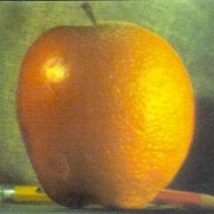
This is my second project for CS 180 (Intro to Computer Vision) at UC Berkeley. The project goes over how filters work in image processing and how we can manipulate images in the frequency domain to get interesting effects like edge detection, sharpening, and multiresolution blending. Here’s an example of a blended image I made as part of this project:

Part 1: Filters and Edges

Part 1.1: Finite Difference Operator

I implemented a zero-padded 2D convolution operation in NumPy, then compared it with scipy.signal.convolve2d.

Implementation Details

I created two versions:

4-loop version: Explicitly loops through every kernel element
2-loop version: Uses vectorized operations like np.dot

Both implementations produce the same results though the two-loop version is more efficient. One difference from scipy is boundary handling: my implementation uses zero-padding, but scipy.signal.convolve2d has various other options (fill, wrap, symm).

Runtime Comparison

The 2-loop implementation is faster than the 4-loop version due to vectorization. However, scipy.signal.convolve2d is still much faster, probably because it utilizes advanced techniques like FFT to bring down the runtime from O(n^2) - which is my algorithm’s runtime - to O(n log n).

Code Snippets

Two-loop convolution:

def convolve(im, kernel):
    pad_x = kernel.shape[1] // 2
    pad_y = kernel.shape[0] // 2

    padded_im = np.zeros((2 * pad_y + im.shape[0], 2 * pad_x + im.shape[1]))
    padded_im[pad_y : pad_y+im.shape[0], pad_x : pad_x+im.shape[1]] = im

    kernel_flat = kernel.flatten()

    new_image = []
    for i in range(im.shape[0]):
        new_row = []
        for j in range(0,im.shape[1]):
            curr_chunk = padded_im[i : i + kernel.shape[0], j : j + kernel.shape[1]].flatten()
            new_pixel = np.dot(kernel_flat, curr_chunk)
            new_row.append(new_pixel)
        new_image.append(new_row)
    new_image = np.array(new_image)

    assert im.shape == new_image.shape, "Shape mismatch detected!"
    return new_image

Four-loop convolution:

def convolve_slow(im, kernel):
    pad_x = kernel.shape[1] // 2
    pad_y = kernel.shape[0] // 2

    padded_im = np.zeros((2 * pad_y + im.shape[0], 2 * pad_x + im.shape[1]))
    padded_im[pad_y : pad_y+im.shape[0], pad_x : pad_x+im.shape[1]] = im

    kernel_flat = kernel.flatten()

    new_image = np.zeros_like(im, dtype=float)
    for i in range(im.shape[0]):
        new_row = []
        for j in range(0,im.shape[1]):
            res = 0.0
            for m in range(kernel.shape[0]):
                for n in range(kernel.shape[1]):
                    res += kernel[m, n] * padded_im[i+m, j+n]
            new_image[i, j] = res

    assert im.shape == new_image.shape, "Shape mismatch detected!"
    return new_image

Results: Finite Difference Filters

I applied finite difference operators Dx = [1, 0, -1] and Dy = [1, 0, -1]^T:

Top: Dx (horizontal gradients). Bottom: Dy (vertical gradients)

I also tested a 9x9 box filter for smoothing:

Top: My implementation (zero-padding). Bottom: Scipy (default boundary)

Part 1.2: Finite Difference Operator

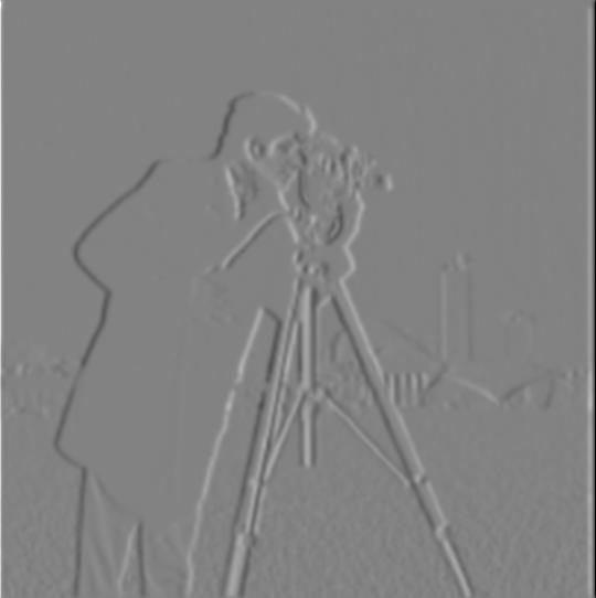
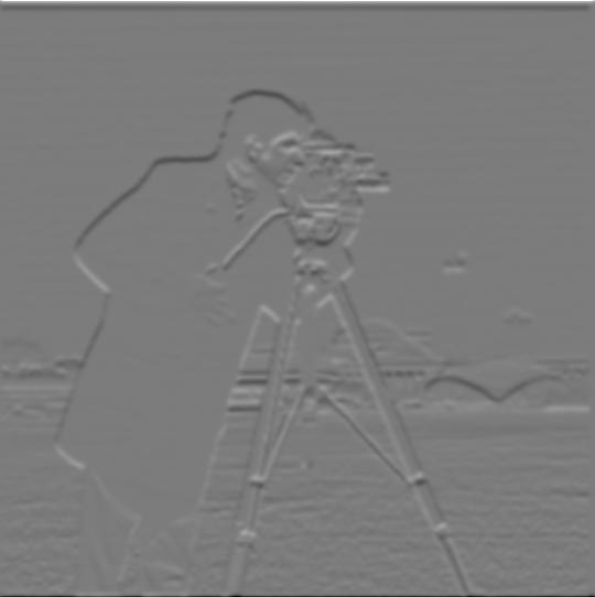
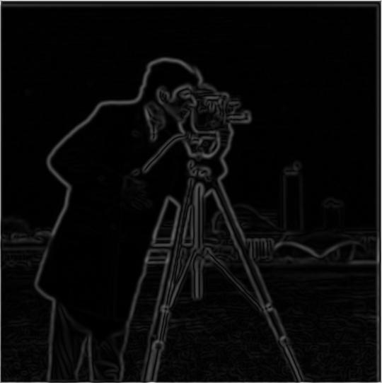
Using the cameraman image, I computed partial derivatives and edge detection with finite differences.

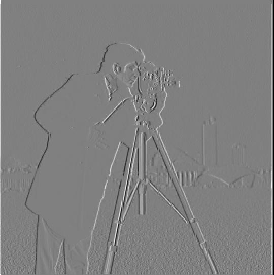
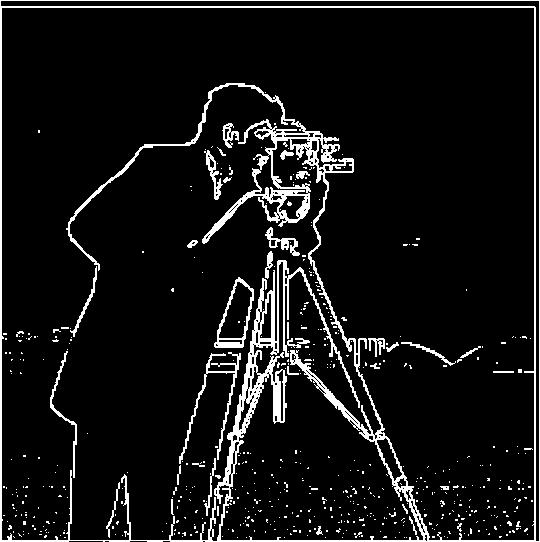
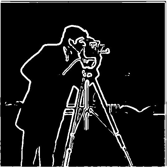
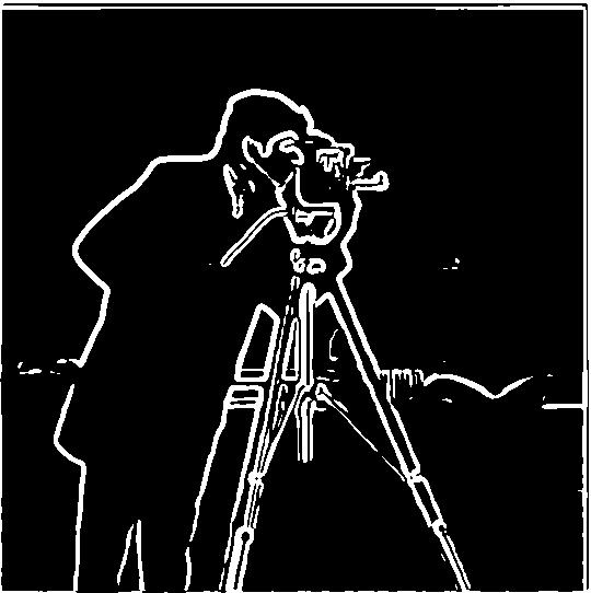
Partial derivatives, gradient magnitude, and binarized edges (threshold=0.20)

The edge image shows significant noise, which is why I had to apply the threshold of 0.20. I chose 0.20 because lower values recorded too much noise in areas like the sky, while higher values removed important edge details in areas like the tripod. A better approach to this problem is to apply Gaussian smoothing first.

Part 1.3: Derivative of Gaussian (DoG) Filter

Background Info

To create the Gaussian kernel, I select a value of sigma, by default 2.0, and then compute the ksize, which I set as 6 times sigma plus one. I then invoke the cv2.getGaussianKernel with these two parameters. In this approach, because ksize is uniquely determined by sigma, I only specify the sigma values when listing the parameters.

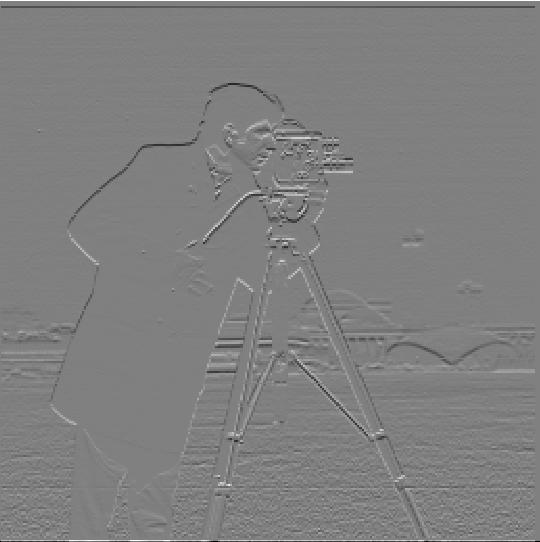
Method 1: Gaussian → Derivative

First blur the image with a Gaussian, then apply finite difference operators:

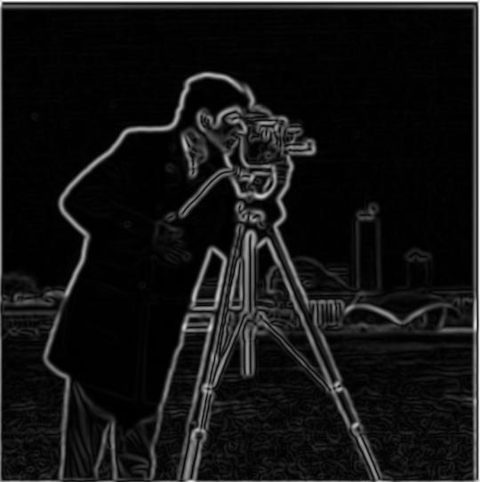
Gaussian blur (sigma=2.0) then derivatives (threshold=0.10) - much cleaner edges!

I chose a threshold of 0.10 by trial and error: I found that it reduced noise without removing too much valuable information.

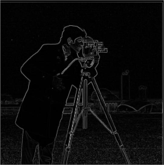
Method 2: Single DoG Convolution

By the property of convolution associativity, we can combine the Gaussian and derivative filters first, then apply to the image in one pass. Using the combined DoG filter gives identical results to applying the two filters separately. The Gaussian filter here uses sigma = 2.0 just like in method 1.

The DoG filters:

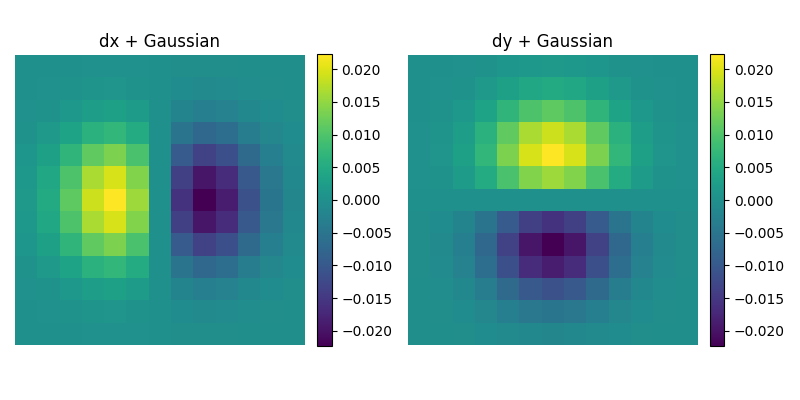
For example, here’s the edge image generated by the combined filter. This produces identical results to Method 1 and demonstrates the associativity property of convolution: (Image ⊗ Gaussian) ⊗ Derivative = Image ⊗ (Gaussian ⊗ Derivative). Results:

Part 2: Applications

Part 2.1: Image “Sharpening”

The unsharp mask filter enhances edges by emphasizing high frequencies. The process:

Blur the image to get low frequencies
Subtract blurred from original to isolate high frequencies
Add scaled high frequencies back: sharpened = original + α × (original - blurred)

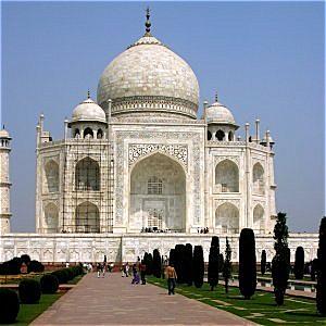
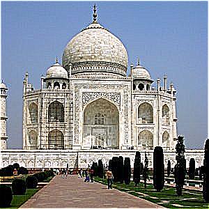
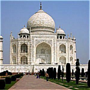
Taj Mahal Results

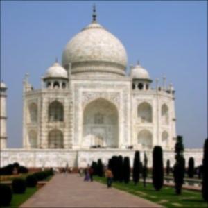
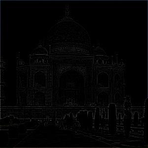
Original, blurred, high frequencies, and sharpened (α=2.0)

Varying Alpha Parameter

α = 0.5, 1.0, 2.0, 5.0 (more α = more sharpening, but also artifacts)

Additional Example

Original and sharpened (α=40.0)

Blur → Sharpen Experiment

Can sharpening recover a blurred image?

Original sharp vs. blurred then sharpened - some detail lost forever

Sharpening helps, but there’s no way to fully recover lost information. Blurring is irreversible.

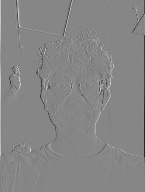
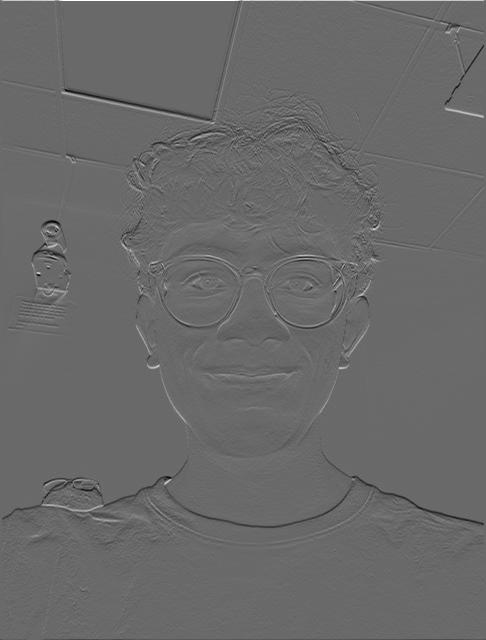
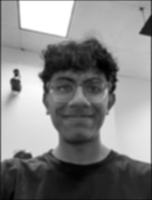
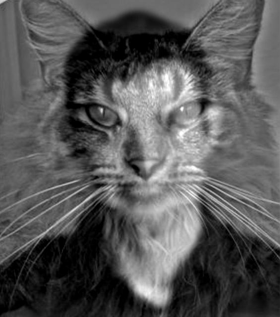
Part 2.2: Hybrid Images

Hybrid images take advantage of how the human eye perceives frequencies at different distances. The technique combines the low-frequency components of one image with the high-frequency components of another. Low frequencies capture broad shapes and overall structure, which dominate our perception from far away. High frequencies encode fine details and edges, which we perceive up close. To create a hybrid image, I apply a Gaussian low-pass filter to extract smooth, large-scale features from the first image, then subtract a Gaussian-blurred version from the second image to obtain only its high-frequency details. When these are combined, viewers see different images depending on their distance from the image: the high-frequency image is seen from close up and the low-frequency one from far away.

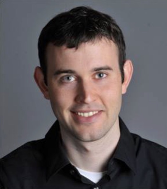
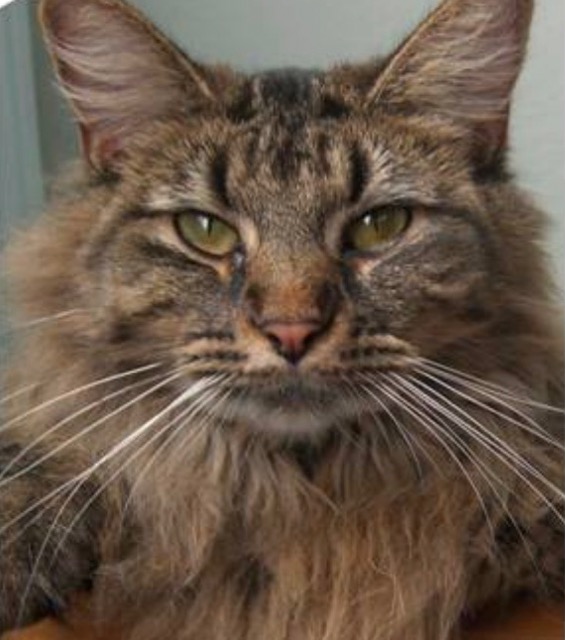
Example 1: Derek + Nutmeg

Frequency Analysis for this example:

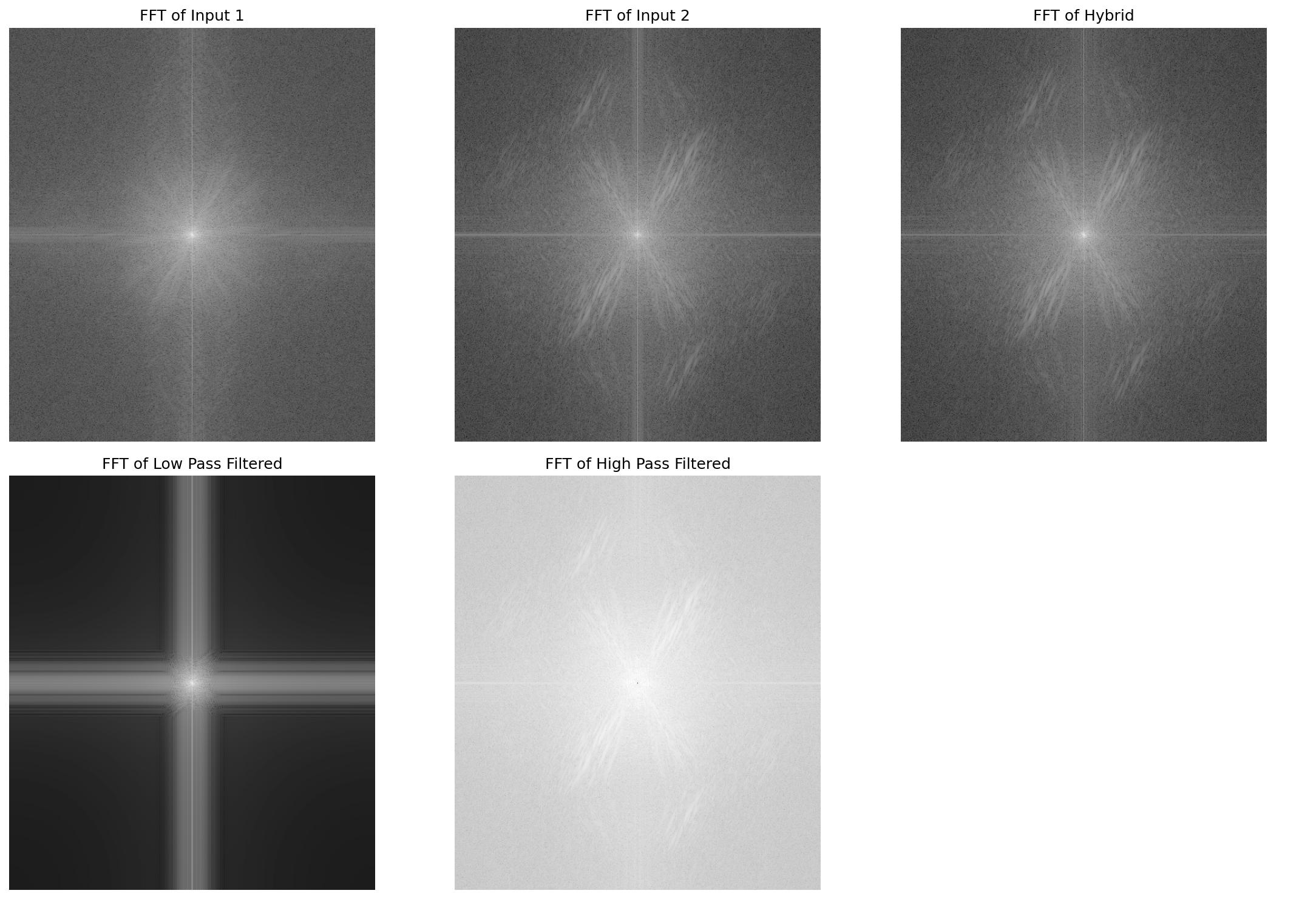
Filtered Results:

For this example, the low-pass Gaussian filter had a sigma value of 15.0 whereas the high-pass Gaussian filter had a sigma value of 6.0. The images were already aligned well, so I performed no manual alignment. (As for the ksize, it is determined by the formula ksize = int(sigma*6.0 + 1).)

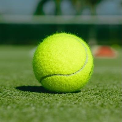
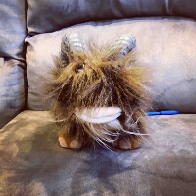
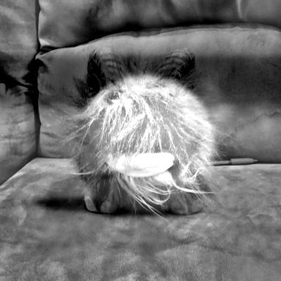
Example 2: Tennis Ball + Monster

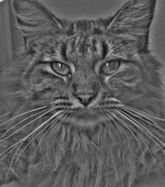
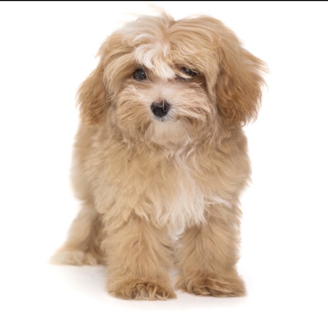
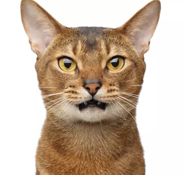
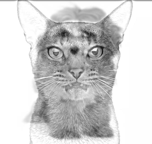
Example 3: Dog + Cat

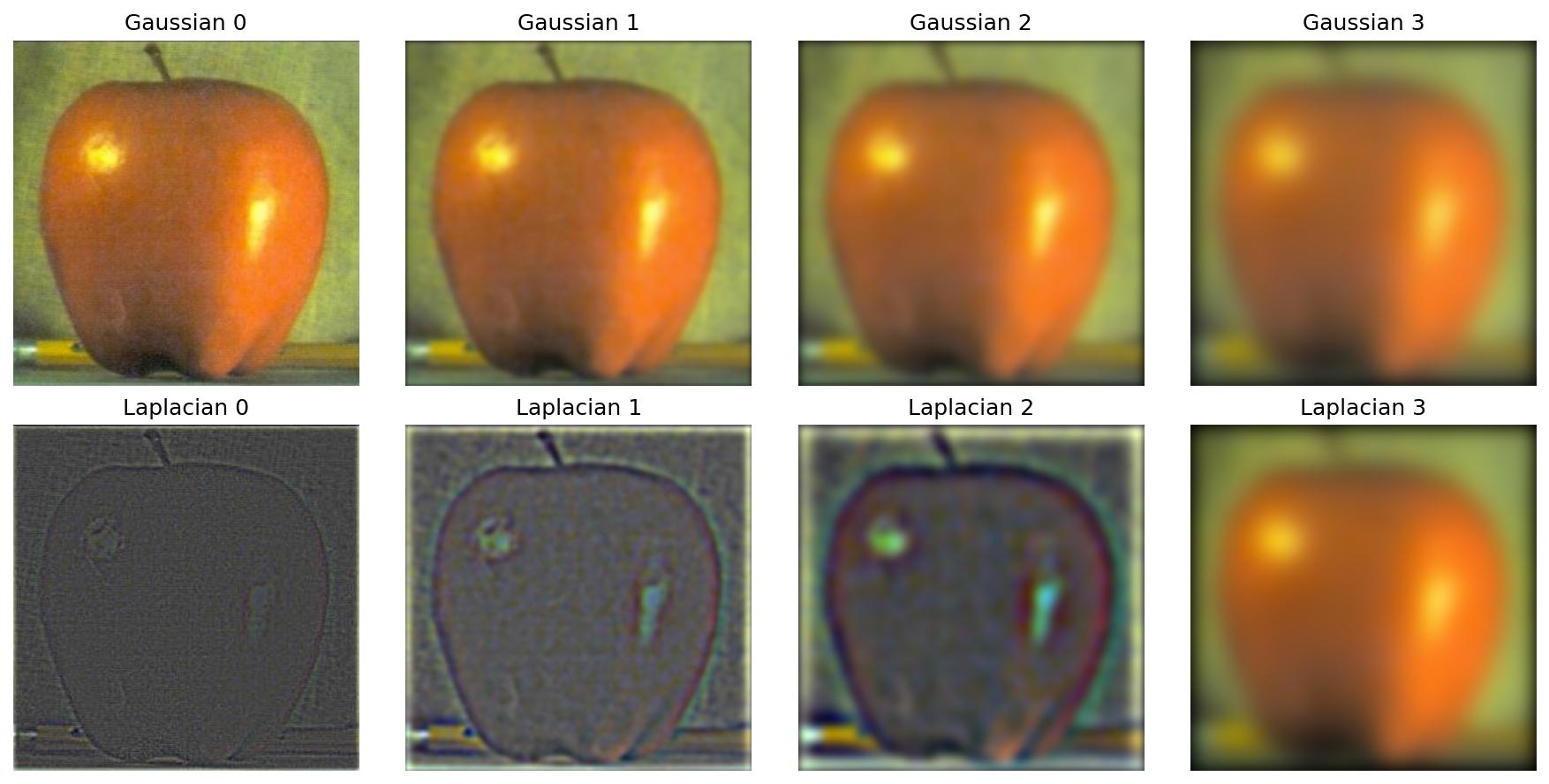
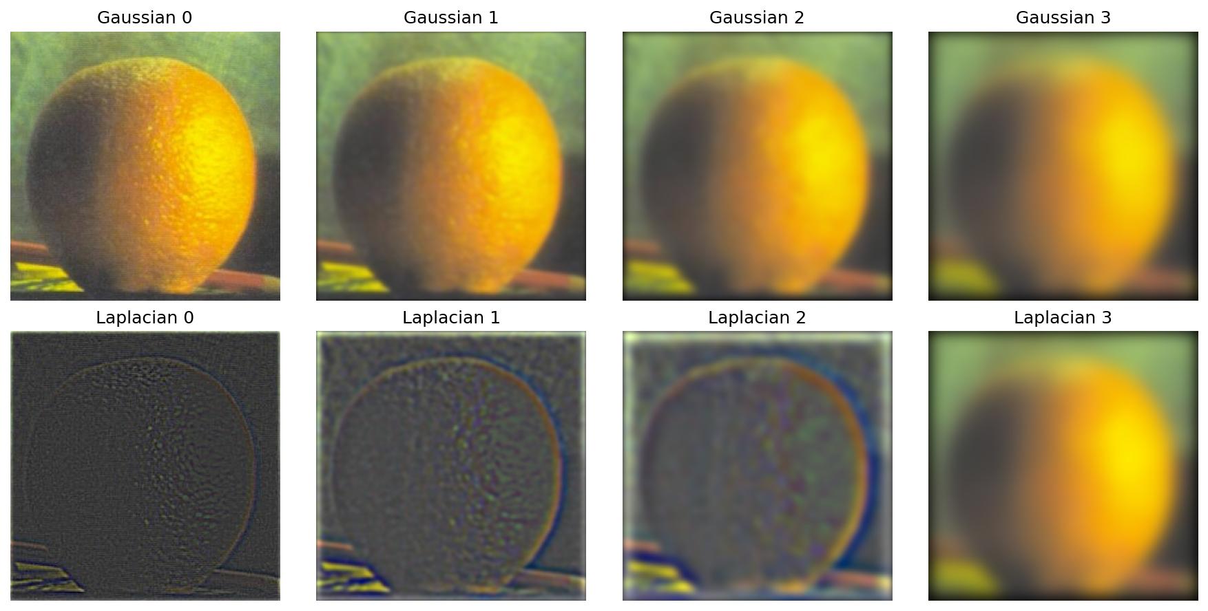
Part 2.3: Gaussian and Laplacian Stacks

Gaussian stacks progressively blur images, while Laplacian stacks capture details at each frequency band.

Apple Stack (for Oraple blending)

Orange Stack (for Oraple blending)

Part 2.4: Multiresolution Blending

Using Laplacian stacks, we blend images seamlessly across frequency bands.

Oraple (Apple + Orange)

Blending Process:

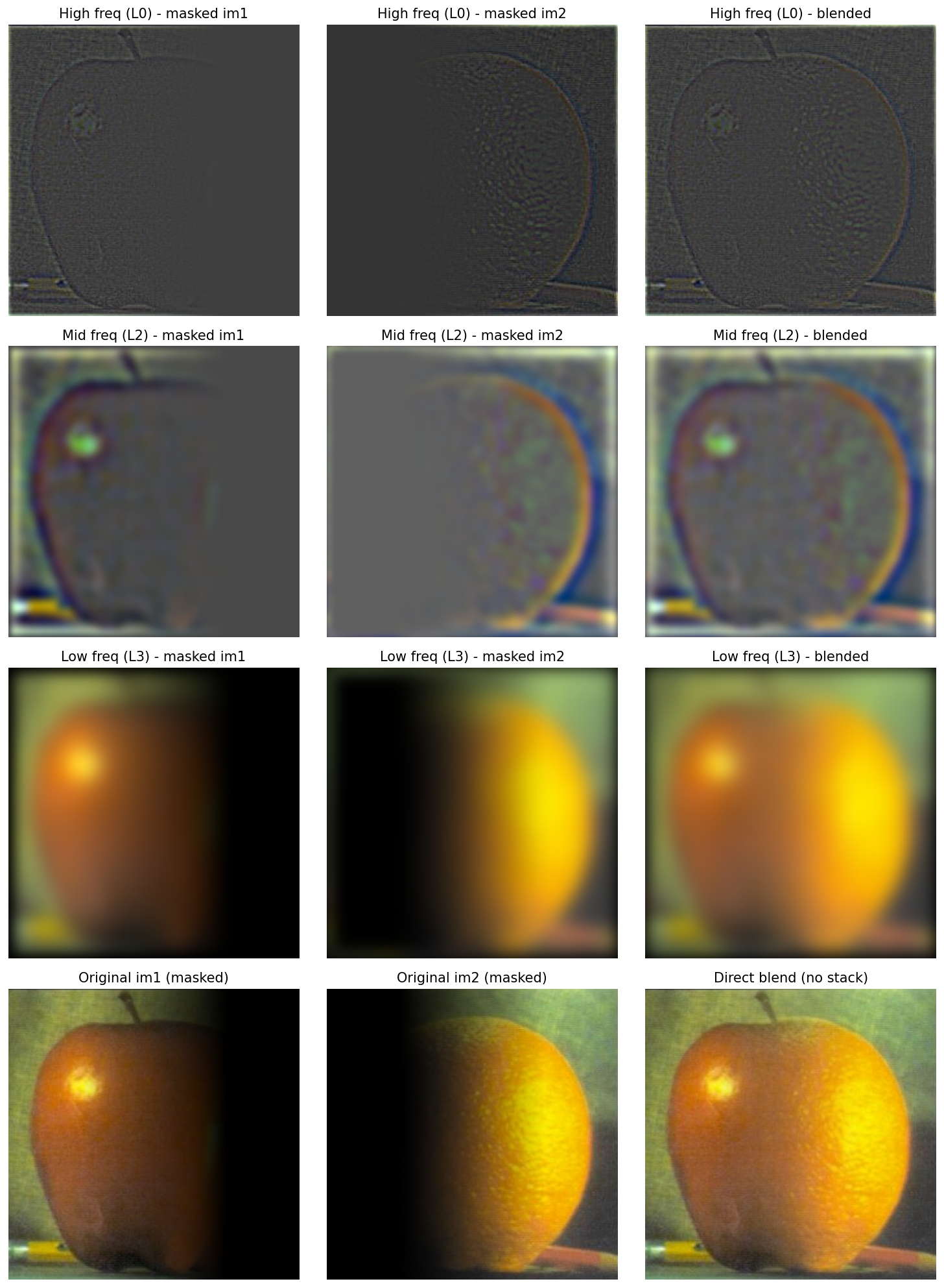
High frequencies show fine details, low frequencies show structure. Here I recreate the outcomes of Figure 3.42 from Szelski

Final Result:

The classic Oraple!

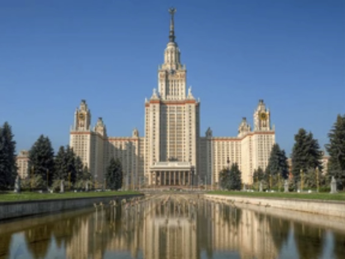
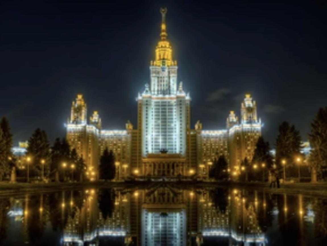
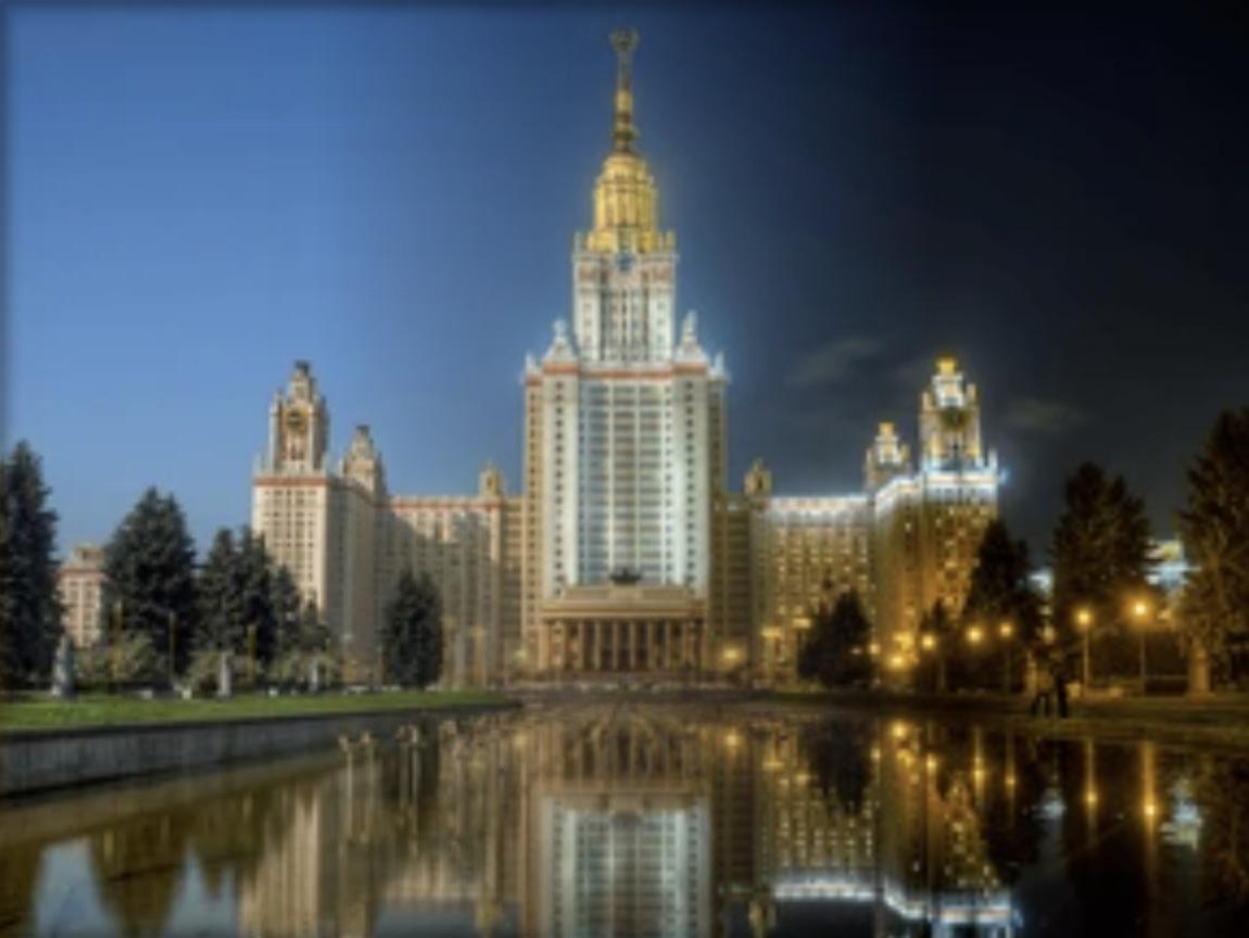
Additional Example 1: Day/Night Blend

Additional Example 2: Irregular Mask + Portal (from Minecraft)

Here I use a circular mask to insert another image inside of the purple portal you see below.

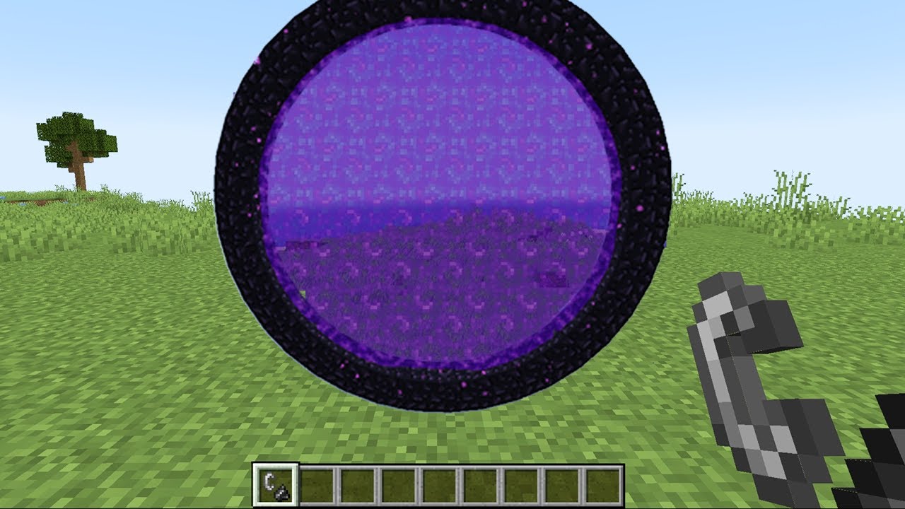
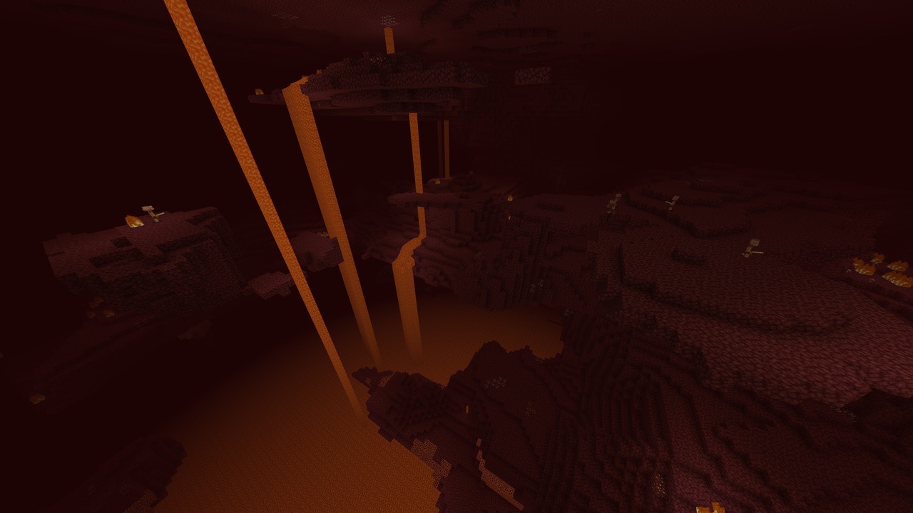
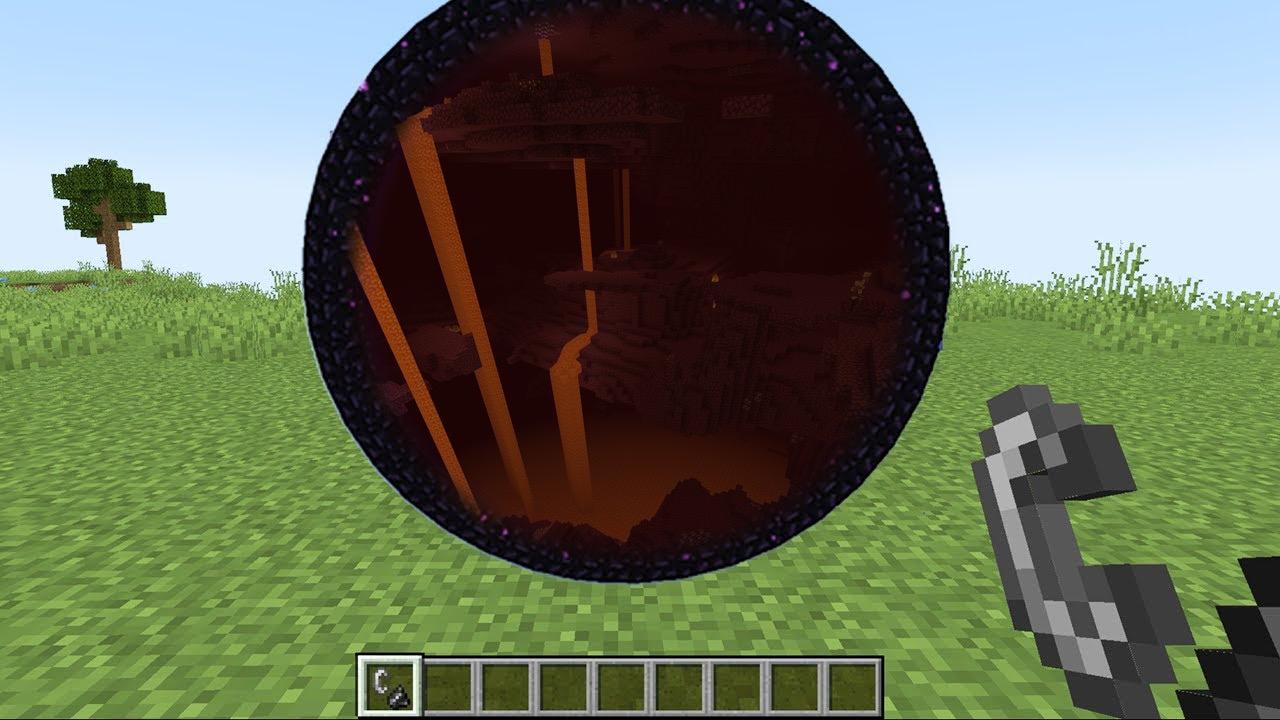
Circular mask creates a portal effect between dimensions

Here’s how the circular mask works:


def make_circular_mask(h, w, center, radius, feather=20):
    Y, X = np.ogrid[:h, :w]
    dist = np.sqrt((X - center[0])**2 + (Y - center[1])**2)
    mask = np.clip((radius + feather - dist) / feather, 0, 1)

    return mask

I experimented with different input arguments to generate the mask and eventually I settled on a center of (630, 280) and a radius of 265.

Most Important Thing I Learned

The most important thing I learned in this project is that classical methods are still very useful in 2025. These days neural network-driven approaches are very popular in the CS world, and rightfully so, but this project shows us that sometimes it doesn’t hurt to go old-school. For example, we could have used generative AI to merge the orange and apple photos, but there’s no reason to do that when the multiresolution blending approach can get the same result with a fraction of the resources.