Generating Image Mosaics (and more!)

08 Oct 2025

Introduction

This is my third project for CS 180 (Intro to Computer Vision) at UC Berkeley. The project covers image warping, image mosaic generation, and automatic feature detection for image stitching.

Part A.1: Shoot the Pictures

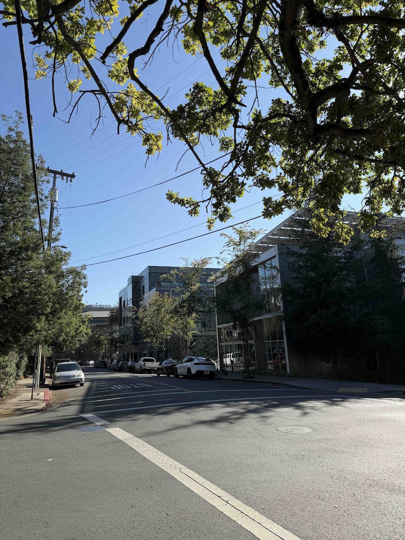
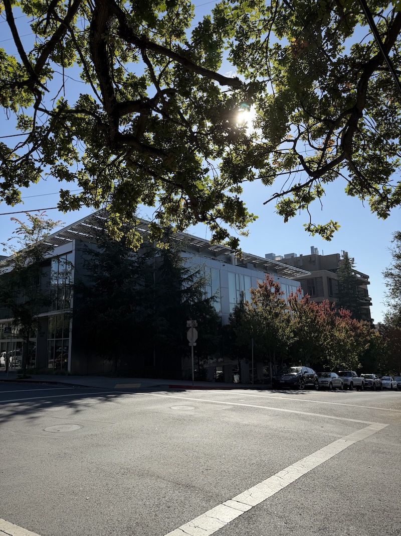
The first part of the assignment is to show at least 2 sets of images with projective transformations between them (fixed center of projection, rotate camera). The reason we are doing this is because we can then use these images to construct mosaics later on in the assignment.

Set 1:

Set 2:

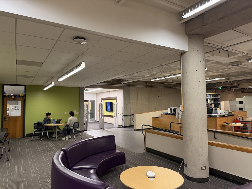
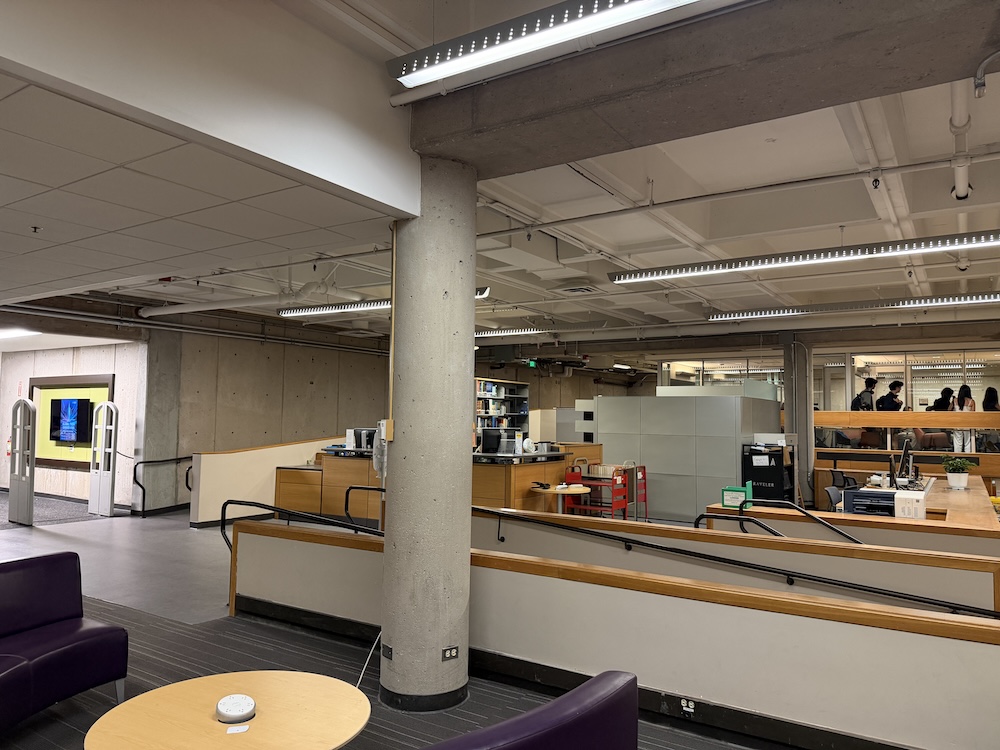
Notice how the camera position is the same in both sets of images; all we’re doing is rotating it. Eventually, we will stitch these images together to create an image mosaic (see part A.4!).

Part A.2: Recover Homographies

A homography is a 3x3 projective transformation that maps points from one image to another when both images capture the same scene.

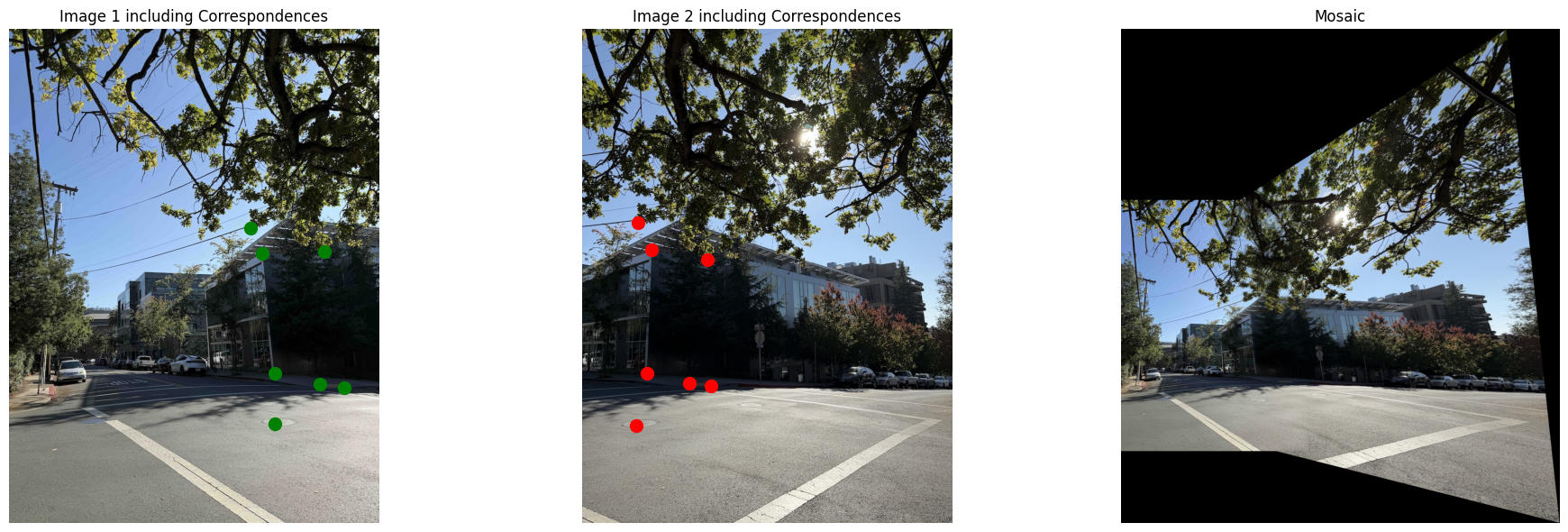
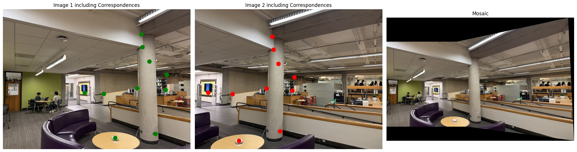
For this exercise, consider the below two images:

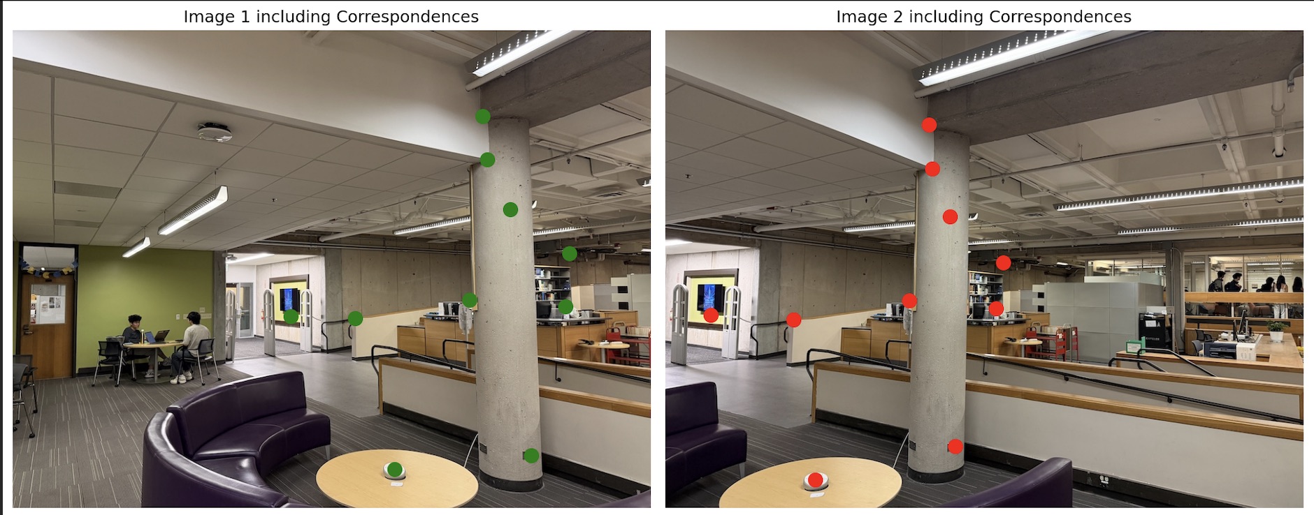
Observe that I manually selected correspondence points between the two images. These are necessary to align the images properly. Only four points are strictly necessary for the algorithm to work, but in practice it makes sense to select many more than four for redundancy.

In homogeneous coordinates: p2 = Hp1, where p1 = [x, y, 1]^T, p2 = [x', y', w']^T, and H is:

[ h11 h12 h13
h21 h22 h23
h31 h32 h33 ]

We convert the system to Cartesian coordinates by dividing by the ‘scaling factor’ introduced by the Homogeneous coordinates:

x' = (h11*x + h12*y + h13) / (h31*x + h32*y + h33)
y' = (h21*x + h22*y + h23) / (h31*x + h32*y + h33)

Rearranging gives two equations per correspondence:

x*h11 + y*h12 + 1*h13 - x*x'*h31 - y*x'*h32 = x'*h33
x*h21 + y*h22 + 1*h23 - x*y'*h31 - y*y'*h32 = y'*h33

Setting h33 to 1 as discussed in class, we arrive at the system of equations:

x' = x*h11 + y*h12 + 1*h13 - x*x'*h31 - y*x'*h32 
y' = x*h21 + y*h22 + 1*h23 - x*y'*h31 - y*y'*h32 

Stacking all pairs yields the linear system Ah = b with
h = [h11 h12 h13 h21 h22 h23 h31 h32]^T. I solved the resulting system of equations using least-squares (because we have >4 correspondences, the system is overdetermined).

This is the homography matrix H which I recovered:

[[ 1.46568340e+00 -1.20053461e-01 -4.98410322e+02]
[ 2.29064746e-01  1.24290079e+00 -1.30462059e+02]
[ 5.01352998e-04 -9.85491138e-05  1.00000000e+00]]

Part A.3: Image Warping and Rectification

In this section, I use the recovered homography H to warp images toward a reference view using inverse warping.
Inverse warping maps each pixel in the output image back into the input image coordinate system. This prevents holes or “gaps” in the outputted image.

1) Warp Functions

After we inverse-warp the image, there’s a problem: the resulting coordinate values are not integers! There are many kinds of interpolation methods we can apply to address this problem. Here I discuss two interpolation methods that I implemented from scratch.

Nearest Neighbor Interpolation: Round coordinates to the nearest pixel value. Runs relatively quickly but the results aren’t as good as bilinear interpolation.

Bilinear Neighbor Interpolation: Use a weighted average of four neighboring pixels. Takes longer but gives better-quality results.

2) Results

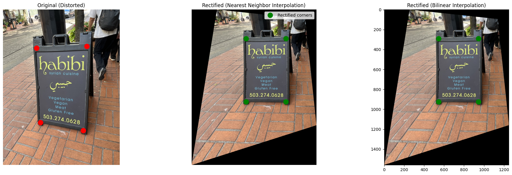
In the below image, zoom in on the words “vegetarian” and “vegan” on the sign. Notice how the bordering around the letters is less jagged and pixelated in the bilinear interpolation image, compared to nearest-neighbor.

Here’s another example:

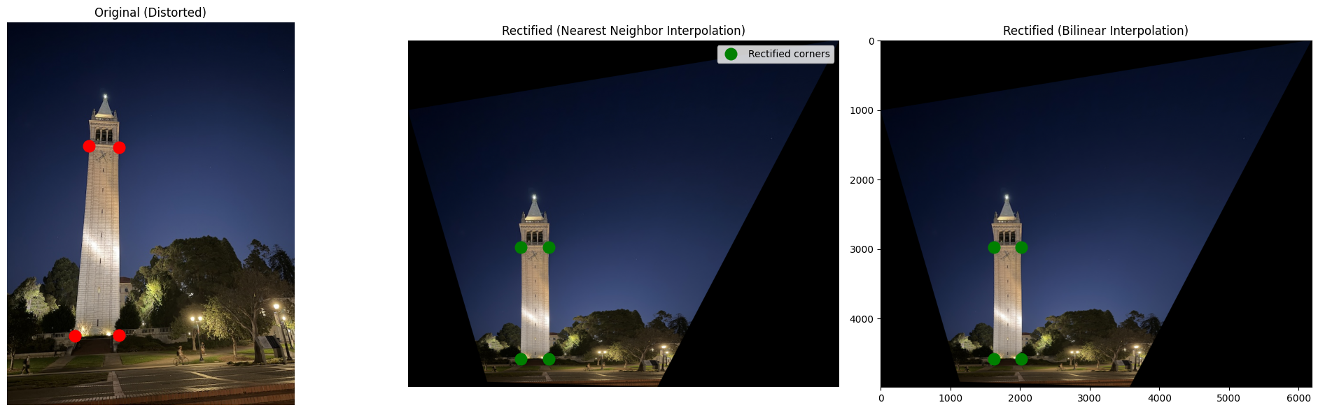
For these examples, there is no ‘‘second image’’: instead, we warp the first image to a predetermined shape (a rectangle).

For the campanile example, I set the second image’s coordinates to that of a rectangle with height four times that of the width. Here’s what the coordinates of that rectangle looked like, for reference:

  "im2Points": [
    [0, 0],
    [1, 0],
    [1, 4],
    [0, 4]
  ]

For the sign image, I used a rectangle with height 1.58 times the width. I determined these values through manual measurement of the image and trial and error.

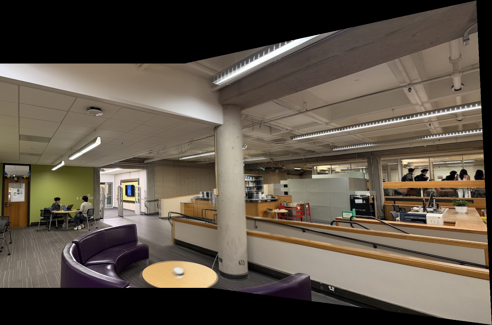
Part A.4 Blend the Images into a Mosaic

In this next part, I developed an algorithm to stitch images together into panoramas!

Procedure (one-shot, inverse warping)

Choose reference: Leave one image unwarped and warp the other into its projection using the computed homography.
Create alpha masks: For each image, define an alpha mask that indicates which pixels are valid, post-warping.
- Pixels filled during warping are set to 1 (valid).
- Empty or outside regions remain 0. These masks tell you which parts of the canvas belong to which image, and they decide how blending works in areas where the images overlap.
Apply weighted averaging to reduce artifacts: To smooth the overlap between the two images, I gave each pixel a weight based on how far it is from the image edge. To accomplish this, I define variables weight_1 and weight_2, where each is computed from the distance transform of its image’s alpha mask:
```
dist_1 = distance_transform_edt(alpha_mask_1) # distance transform method imported from scipy
weight_1 = dist_1 / (np.max(dist_1) + 1e-8)
# dist_2, weight_2 defined the same way
```
Pixels near the center of each image have higher weights, and edge pixels have lower weights. When blending, areas of overlap are averaged accordingly:
```
mosaic = (weight_1 * image_1 + weight_2 * image_2) / (weight_1 + weight_2)
```
This produces a soft, seamless transition between the two images. (In practice, the averaging is applied separately to each color channel, not all at once.)

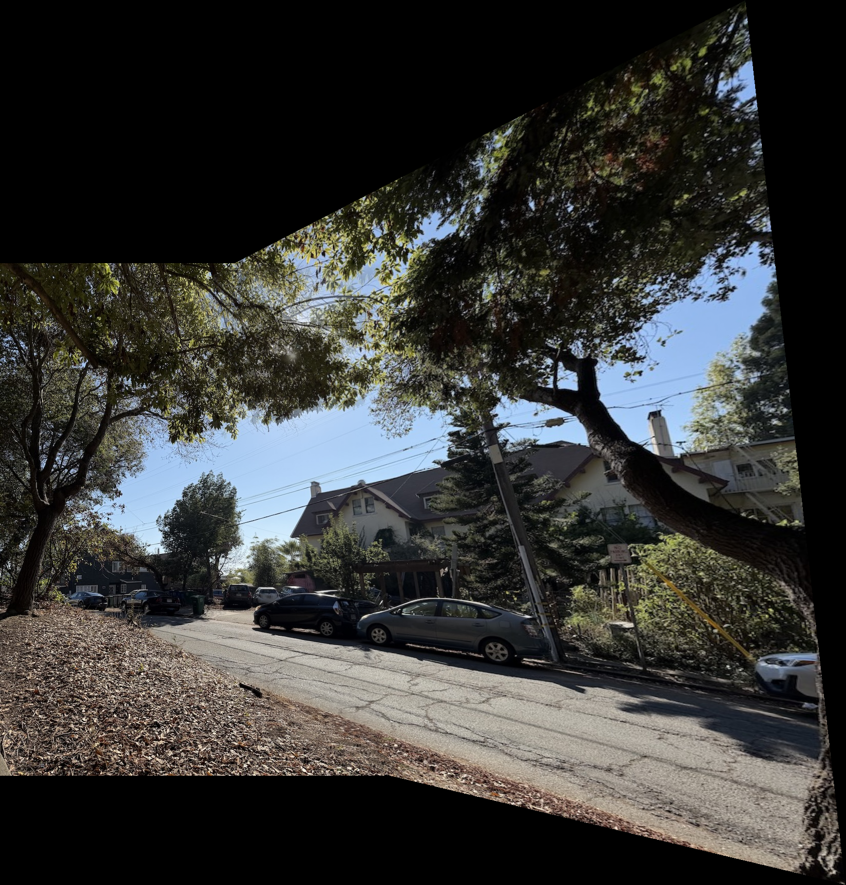
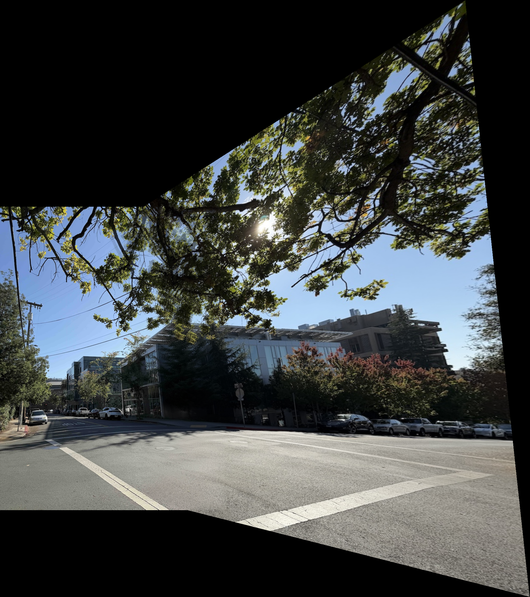
Results

Here are the mosaics with the original images:

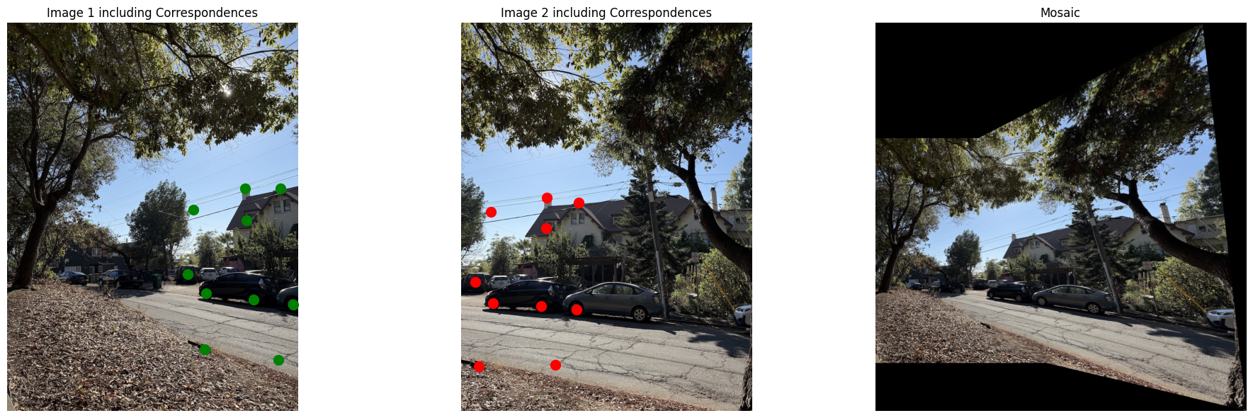
Here are the mosaics on their own for reference:

Part B: Automatic Feature Detection and Matching

In Part A, I manually selected correspondence points to create mosaics. This was tedious and error-prone. In Part B, I implemented an automatic system that detects features, matches them between images, and creates mosaics without any manual input.

The algorithm is based on the paper “Multi-Image Matching using Multi-Scale Oriented Patches” by Brown et al.

Part B.1: Harris Corner Detection

The first step is to detect interesting points (corners) in the image automatically. I used the Harris corner detector to find points with strong intensity gradients in multiple directions.

Here’s the result on a test image with all detected Harris corners:

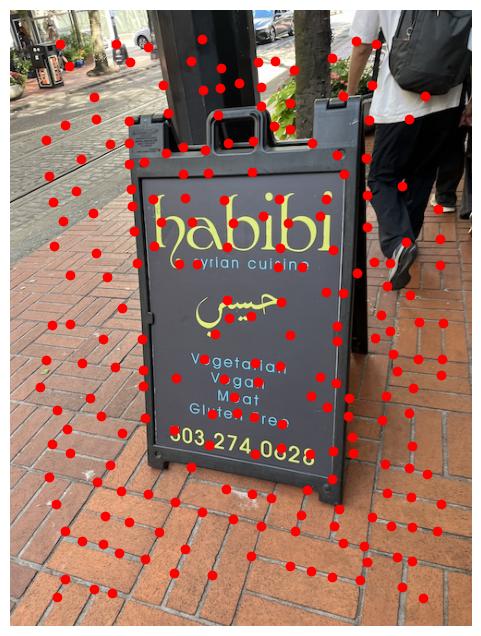
As you can see, there are way too many corners detected.

How can we extract the most important corners and filter out the rest? That’s where ANMS comes in clutch!

Adaptive Non-Maximal Suppression (ANMS)

We use Adaptive Non-Maximal Suppression (ANMS) to get a more uniform spatial distribution of interest points. Each point’s suppression radius depends on its corner strength: points are kept only if they are local maxima within a radius where no stronger neighbor exists. The minimum suppression radius for a point x_i is defined as the distance to the nearest point x_j with significantly higher strength, f(x_i) < c_robust * f(x_j), using c_robust = 0.9.

Here’s the same image after applying ANMS to filter the bad corners.

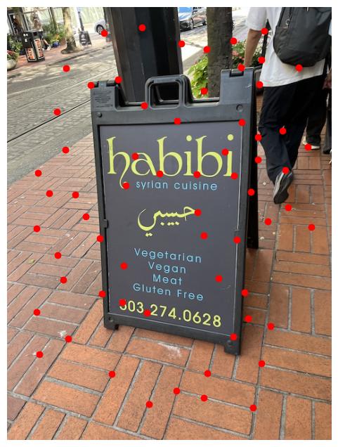
The selected corners are much more evenly distributed and correspond to distinctive features in the image.

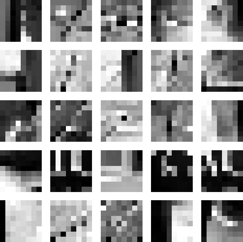
Part B.2: Feature Descriptor Extraction

Once I have corner locations, we need to describe what each corner looks like so we can match them between images.

For each corner, I extracted a 40×40 patch around it, convolved it with a Gaussian filter to blur it (using code from project 2), then downsampled it to 8×8. I normalized each descriptor to have zero mean and unit variance, as is standard practice.

Here are some of the 8×8 feature descriptors I extracted. Each small patch captures the local appearance around a corner point.

Part B.3: Feature Matching

To match features between two images, I compared their descriptors. For each feature in image 1, I found its closest match in image 2 by computing the distance between descriptors.

Of course, not all the matches are good. I used Lowe’s ratio test to filter out bad matches:

For each feature, find the two closest matches
Keep the match only if the closest is significantly better than the second-closest
Ratio threshold: if distance_to_best / distance_to_second < 0.85, keep it

The intuition here is that if you are torn between two options, chances are that neither of them are very good. There should be one option that is vastly better than all the others.

Here are the feature matches I found between two library images:

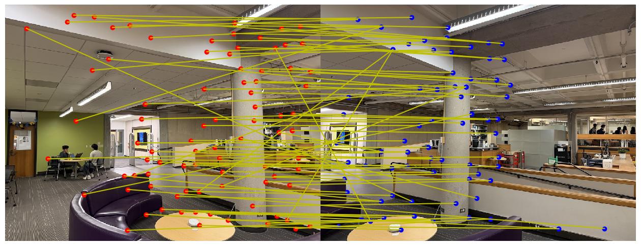
You might have noticed that some of these matches are not good, even with Lowe’s ratio test. But don’t worry! In the next subpart, we will fix this issue.

Part B.4: RANSAC and Automatic Mosaics

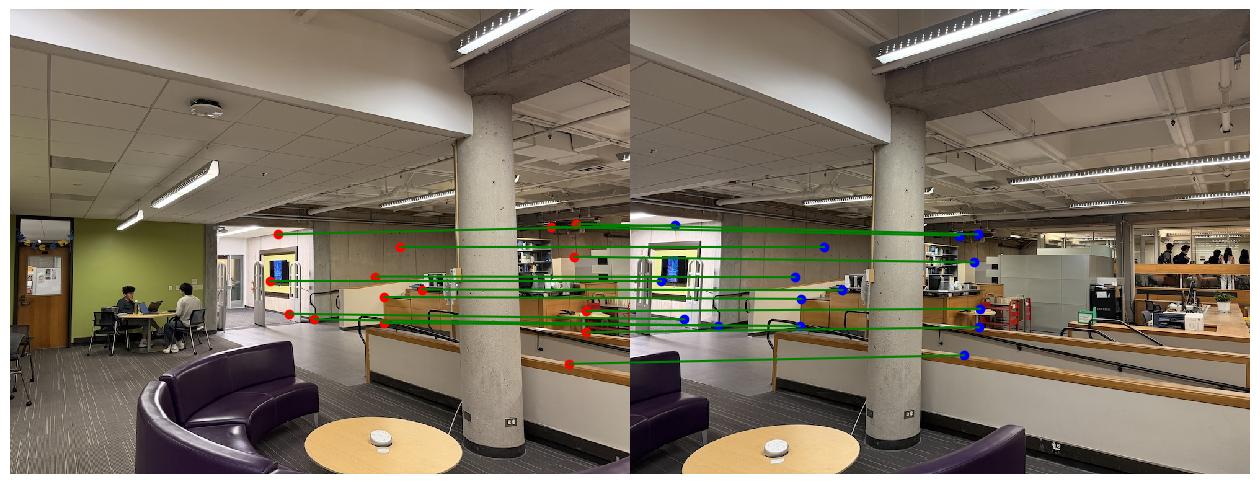
The code we just wrote has a problem - some feature matches are still wrong. We refer to this bad matches as outliers. Conversely, desirable matches (ones that are correct) are called inliers. We want to compute the optimal homography using just the inlier points, not the outliers. That’s where we use RANSAC: Random Sample Consensus, an interesting algorithm that actually has many applications beyond just image processing.

How RANSAC Works:

Randomly sample 4 feature correspondences
Compute a homography from these 4 points
Count how many other matches agree with this homography (or are reasonably close)
Keep largest set of inliers
Recompute the final homography, using just the inliers

Here are the matches after RANSAC filtering (only inliers shown):

Automatic vs Manual Mosaics

Now, we can create mosaics automatically, without painstakingly labeling correspondences. Here’s a comparison of manual stitching (Part A) versus automatic stitching (Part B) on the same image pairs:

Library Mosaic:

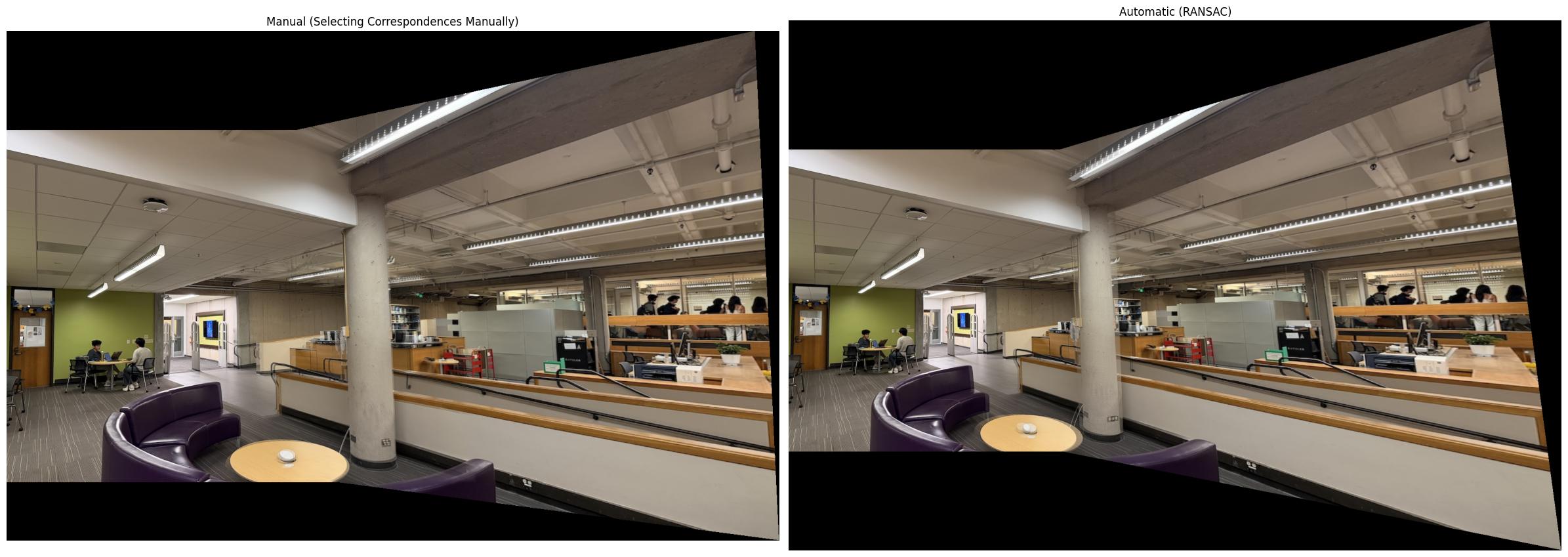
Northside Mosaic:

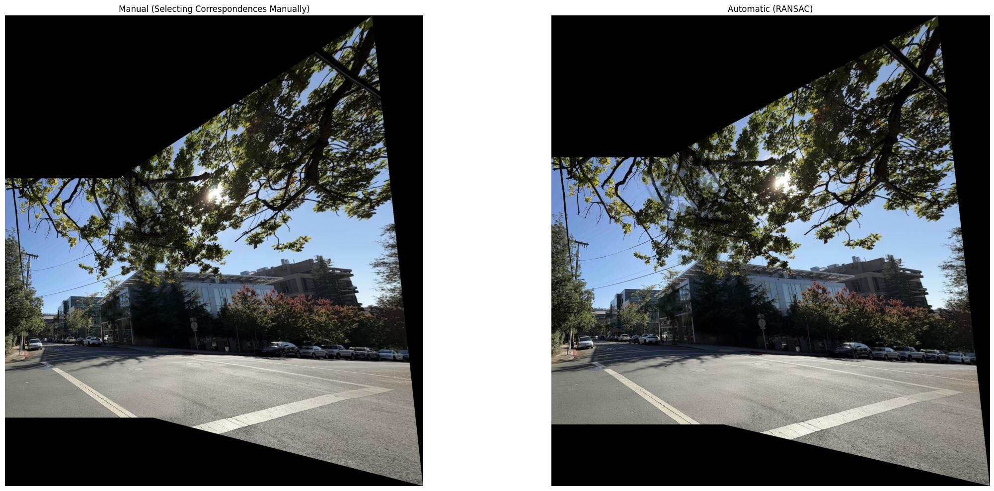
Road Mosaic:

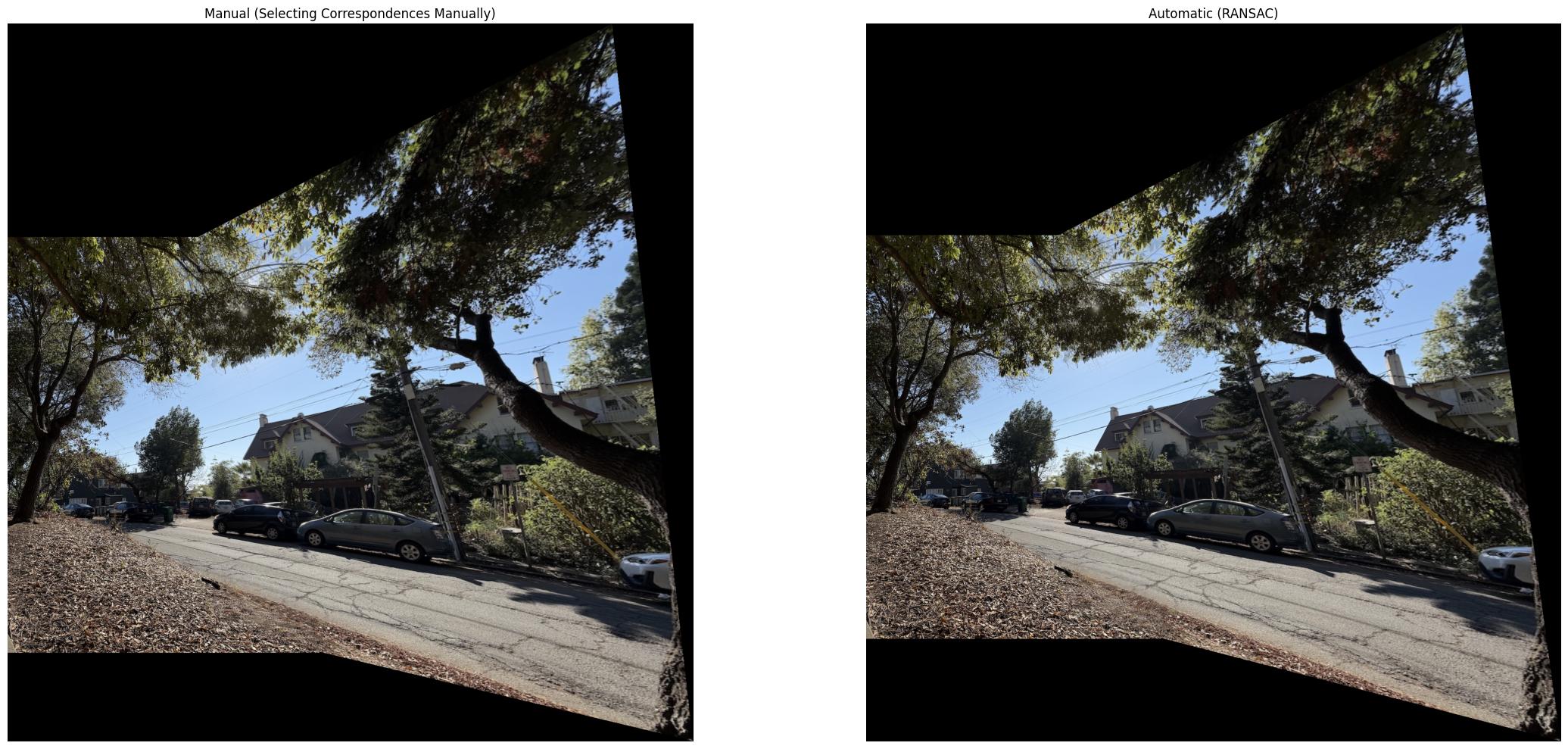
One key takeaway here is that RANSAC achieves pretty good results! The manual mosaics are better in a few spots, but given that RANSAC doesn’t have access to the manual correspondences, I think it did well.

What I Learned

The biggest takeaway I got from this project was the importance of filtering heuristics: algorithms / techniques for turning a large, messy set of features into something actually useful. An example of a “filtering heuristic” would be Lowe’s ratio test, as well as ANMS. The intuitions behind why we filter out certain points and keep others are definitely something that generalizes beyond image processing. As I continue in my ML journey, I will keep in mind these broad takeaways.