Implementing NeRFs (Neural Radiance Fields) from scratch
TLDR
In this project, I implemented NeRFs (Neural Radiance Fields) from scratch. NeRFs allow you to create 3D “reconstructions” of images, like the one below, using just ordinary photos that you take with your camera.
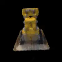
Basically, you take a bunch of photos of an object from various angles and it reconstructs a 3D radiance field of the object.
Background Info
This Fall 2025 semester, I’m taking a computer vision class, titled CS 180, taught by Professors Alexei Efros and Angjoo Kanazawa at UC Berkeley. The task for this project is to implement NeRFs, which are basically a way to synthesize a 3D scene from a set of 2D images. This post will walk you through my whole process of training a NeRF1, from the dataset collection and camera calibration to the actual training of the neural net.
Part 0: Camera Calibration and 3D Scanning
The first task of the project is to take photos of our object from various angles, and place an object called an ARUCO tag next to them. (We are collecting the training data that will be used to train the NeRF later on.)
We also take photos of the camera setup without the object in frame. This is important because it allows us to recover the camera intrinsics. Once we have the camera intrinsics and a bunch of photos of our object,
we pass it into a method that undistorts the images, computes camera-to-world (c2w) matrices, and splits the photos into train, test, and validation images.
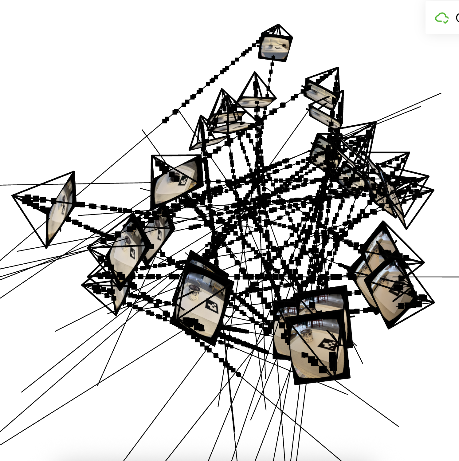
Here is a visualization of the camera frustums recovered by my code from two different angles:
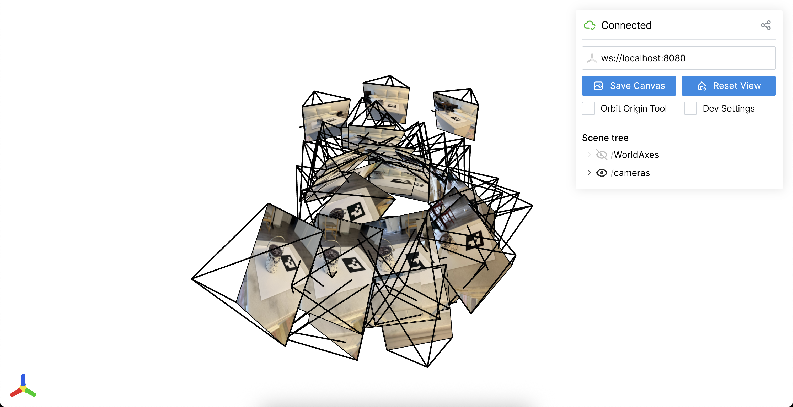
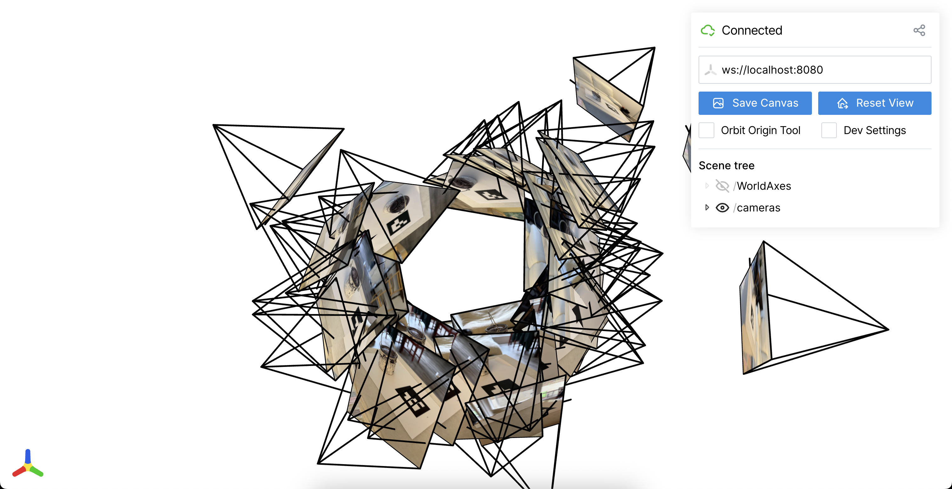
One thing I’d like to note is that setting the tag length to 60mm, which is its actual length, does not give good results because the markers end up too far apart.
For this reason, my code assumes tag_length = 0.6 instead of tag_length = 60.
Part 1: Fitting a Neural Field to a 2D Image
Our first, warmup task is to fit a neural field to a 2D image.
This isn’t used to create our NeRFs, but it’s a helpful exercise to get us familiar with the libraries
that we will be using in part 2.
If you can understand the 2D case well, then it’s easier to generalize to 3D.
For the single-image regression task I kept the starter MLP that predicts RGB values from positional encodings of (x, y) coordinates.
This is the model architecture:
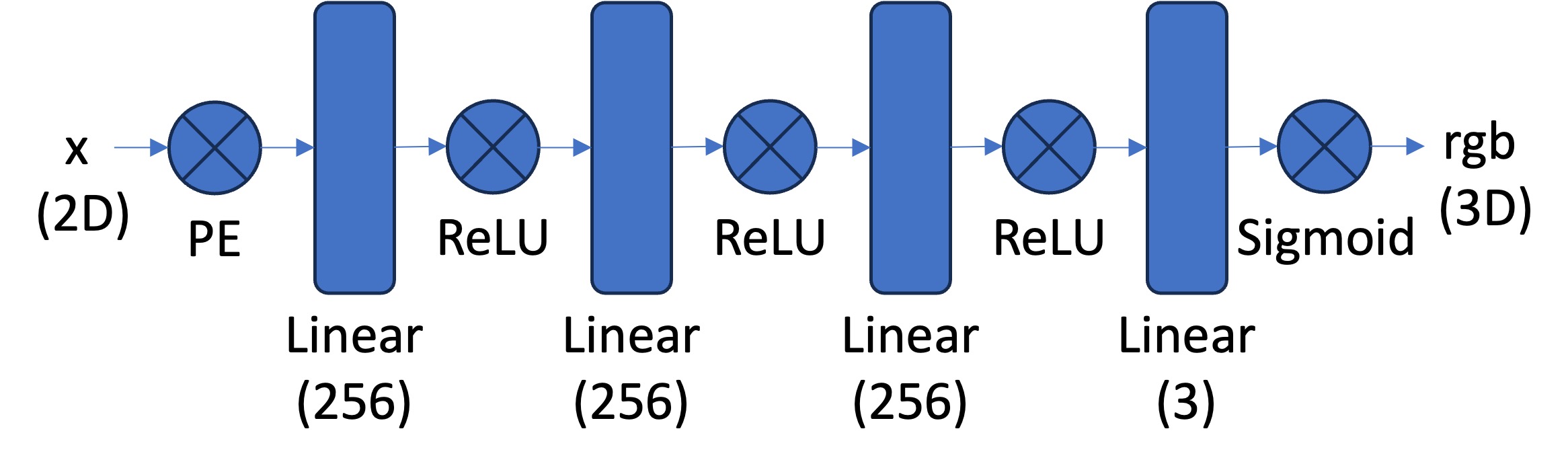
I trained my network using Adam as the optimizer with a learning rate of 1e-2 for 1,000 iterations with a batch size of 10k, as stated in the assignment instructions.
All other hyperparameters were the same as the ones described in the spec.
I also evaluate PSNR every 50 iterations and put that in a separate graph which you will see later in the post.
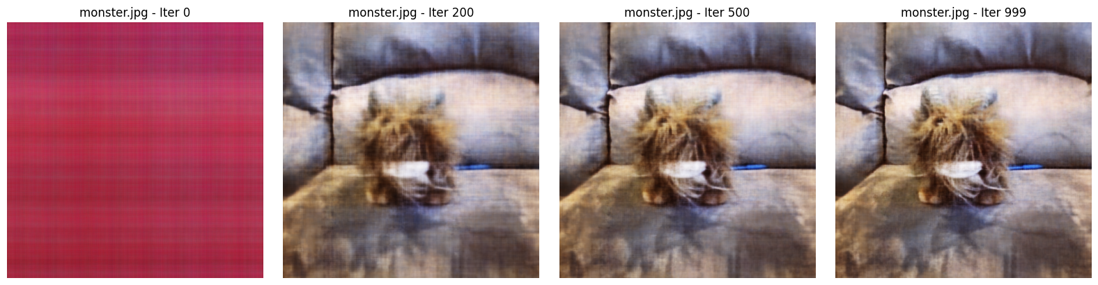
Training progression
The provided “monster” target converges quickly. This makes sense, as the image was relatively simple to begin with.
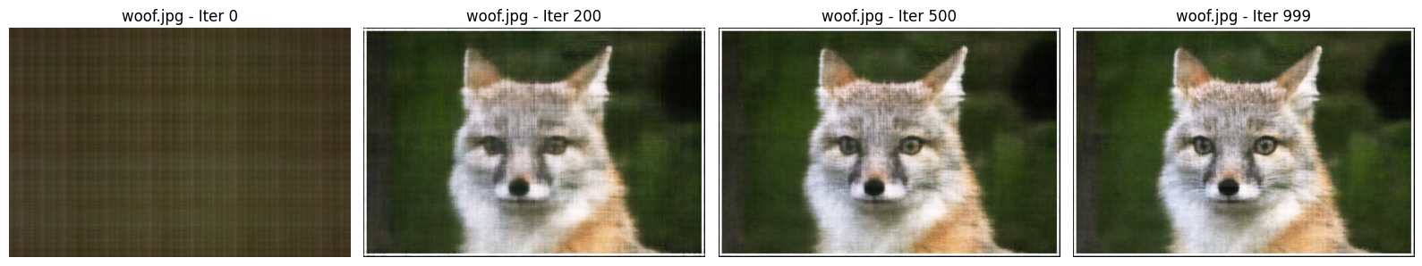
The fox image shows a similar pattern:
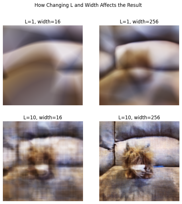
Effect of positional encoding frequency and width
Here we try various values of L and the hidden layer width and put them in a 2x2 grid. This helps us understand how varying the hyperparams affects the overall predictions of the model.
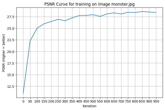
PSNR over training
The PSNR curve shows rapid gains for the first ~200 iterations. This makes sense because the model is learning the lower-frequency, coarse structure of the image. Then it gets smaller improvements as it corrects the higher frequency errors.
Here is the PSNR curve for the custom image (monster.jpg):
Overall, even this simple MLP can overfit a single view pretty well as long as you choose the right hyperparameters.
Other Notes
One optimization that I added is that we precompute the positional encoding of all the coordinates sampled during renders. Recall that we render a model prediction (as seen in the training progression diagram), you have to evaluate the model at many image coordinates to reconstruct its prediction. This requires computing the positional encoding for each coordinate. But since these positional encodings are not learned parameters, we can compute the positionally-encoded version of every pixel in the render ahead of time, which speeds things up a bit.
There are definitely more optimizations we could have done for this part, but as Part 1 is not the main focus on the assignment, I moved on as soon as I got it to work with a reasonable runtime.
Part 2: Fitting a Neural Radiance Field from Multi-view Images
How I implemented each part
With the calibrated cameras from Part 0 in hand, I reconstructed a full NeRF volume for the Lego scene.
Here is the architecture that I used for my neural network, as per the assignment spec:
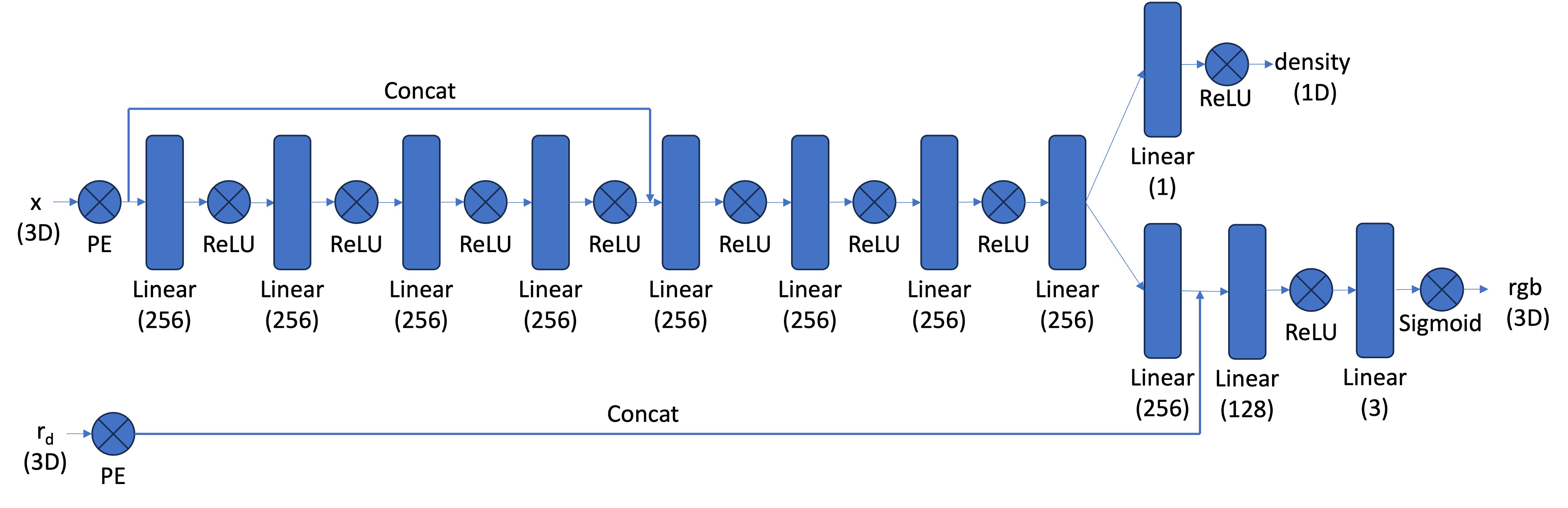
Parameters: The layers and activation functions are all the same as the architecture described in the spec. I set the positional encoding for the X dimension to have L=10, and for the depth r_d, to L=4
Vectorized Code
I feel like the most crucial part of this section is correctly implementing the core methods: volumetric rendering, sampling points along rays, etc: implement these methods correctly and the training loop is generally straightforward (and doesn’t take too much added code).
At first I implemented some of these methods with numpy, but I found that this made training too slow and was too complicated. It required moving too many objects back and forth between my MPS backend and the CPU.
Instead, I implemented all the methods for sampling, dataloading, etc. in PyTorch, and I added support for batched operations. This made my implementation cleaner and easier to understand and debug.
Dataloader Class
I also found it helpful to create a Dataloader class to abstract away some of the complexities of sampling rays from images.
My dataloader init’s method precomputes ray origins and directions for pixels u, v in each image.
This is similar to what we did in part 1: it speeds up training and cuts down on redundant computations.
Other Abstractions
I created helper methods such as nerf_forward_pass, render_full_image and make_renders and housed them in a separate file called pt2_utils.py.
Given the overall complexity of this project, I found it necessary to separate the code into multiple files and maintain helper methods to avoid code repetition.
Visualizing rays and samples
As per the assignment spec, I visualize rays and sample points as a sanity check to make sure my code worked:
Here is a visualization for just one camera:
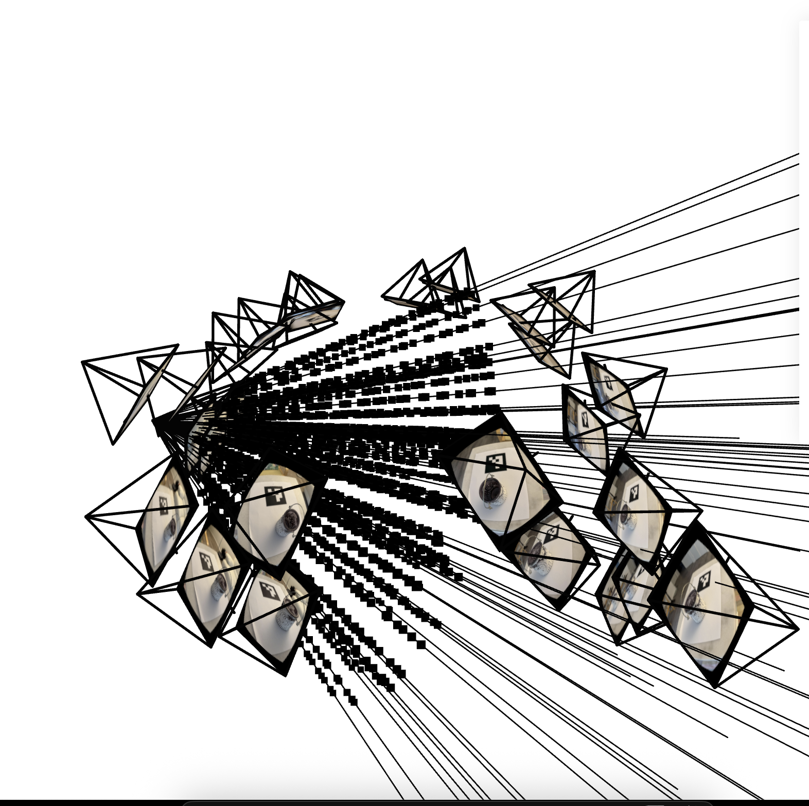
where the darker dots along the lines represent points at which we sample.
As mentioned, we insert a small amount of noise to the sampling intervals in order to improve the model’s predictions. This is somewhat noticeable in the visualizations above; the gap between individual sampling points is not perfectly constant - and that’s by design.
Training progression
The snapshots below capture the predicted RGB image for a validation camera every ~200 iterations.

Validation curve
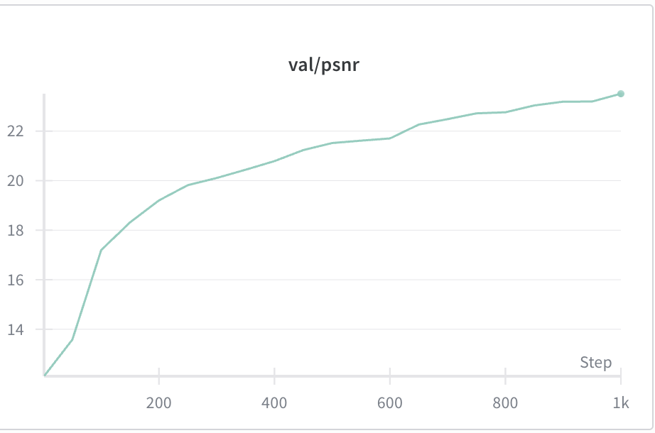
I average the PSNR across six validation images to compute the validation PSNR.
The final PSNR that I achieved was 23.51.
Here is the PSNR curve on that validation set:
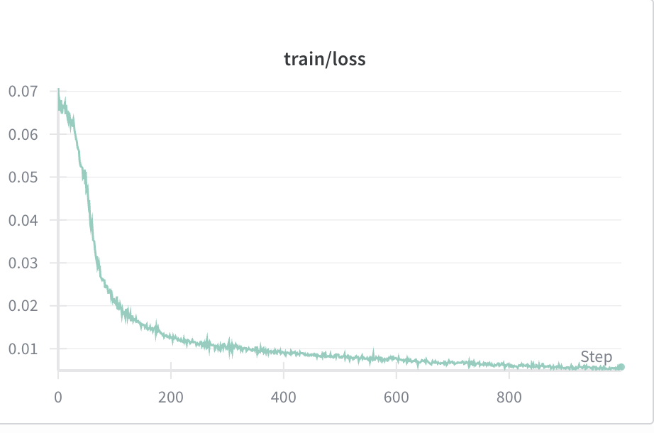
Here’s the training loss curve too:
Spherical rendering
After convergence I evaluate the network across a 360 degree camera path using the provided rendering code.
I use a held-out C2W matrix from the test split (c2ws_test) for this part.
Here is my spherical rendering:
If the rendering isn’t showing, you can also view it at this link: https://www.vkethana.com/assets/images/nerf/pt2/lego/final_gif.gif
Honestly, I thought the results were pretty good given the limited amount of compute / train time we used for this assignment!
Training with my own data (Part 2.6)
After succeeding on the LeGO image, I moved on to making a NeRF with my own set of images.
Unfortunately, this part of the assignment did not go as well :(
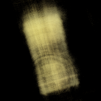
Here is the best spherical rendering that I could achieve:
If the rendering isn’t showing, you can also view it at this link: https://www.vkethana.com/assets/images/nerf/pt2/my_data/final_gif.gif
The model definitely learned something, and you can kind of make out distinct features of the scene in which I took the images, but overall, I would say it was unsuccessful.
Training and PSNR Plots
Here is my PSNR curve, which reached a maximum of value of 10.74 during training.
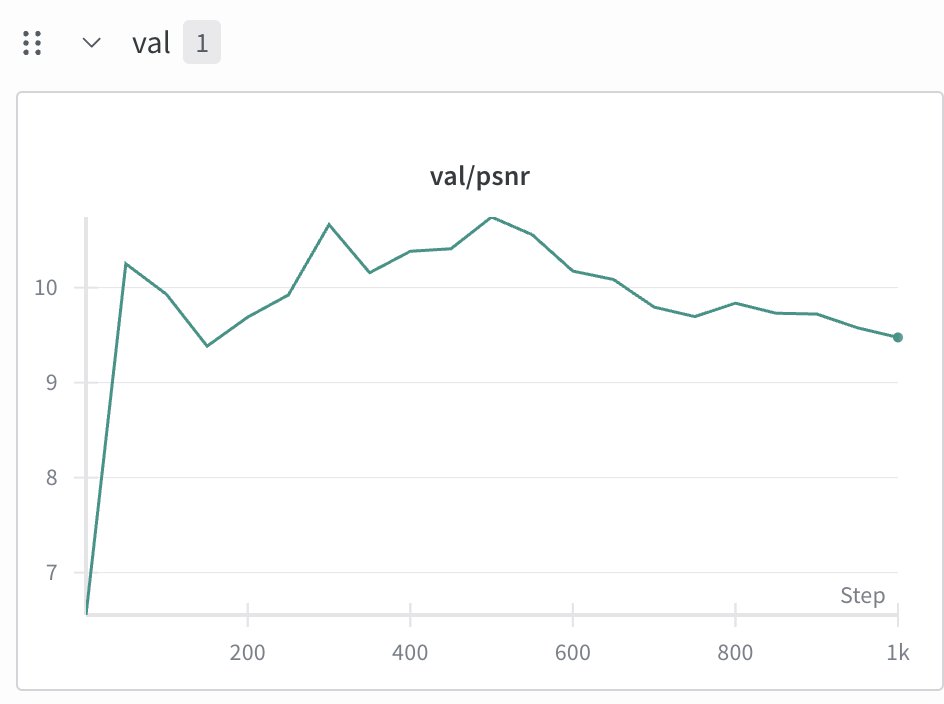
On the bright side, the model did at least show convergence as seen in the below training loss graph:
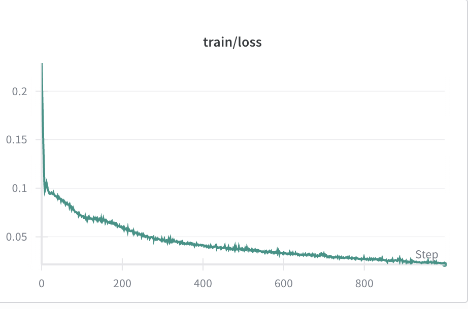
This suggests that the loss landscape just wasn’t shaped properly, i.e. that we need to take better photos or change something about the model architecture.
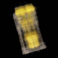
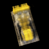
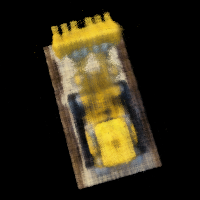
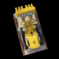
Training progression
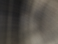
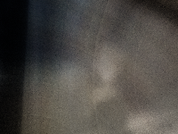
The snapshots below capture the predicted RGB image for a validation camera every ~200 iterations.

Code / Hyperparameter changes made
- I downsized my images from 1500 by 2000 to 150 by 200 in order to prevent OOM errors and speed up training.
- Recall that the original LEGO images were 200x200, so it makes sense for these images to be in roughly the same neighborhood of size
- I use a different set of hyperparameters: I set the positional encoding for
Xto have L = 40 and the positional encoding fordto have L = 15. I chose these experimentally. - Additionally, I set
nearandfar(which determine the distances at which we sample points on the rays) to0.1and2.0respectively. I made this change by looking at the rays/frustum visualization and trying different values until the length / spacing of the sampled points looked reasonable.
Speculation on why my model didn’t work for the custom image: The Data
My guess for why the model did not work very well is that the input images simply weren’t good enough: I could have taken photos from more angles to remediate this.
Additionally, I think it would have been good to shoot images that were closer up, given the small size of the object.
Using a small, black-and-white object may have also been a mistake, because many other objects in the scene were white:
- the white tabletop that I placed it on
- the white piece of paper beneath it
- the white wall / couch in the background of some of the images
Conclusion
One key takeaway I got from the project was the importance of datasets in machine learning. The model architecture here was relatively straightforward to implement based on the assignment instructions. Most of the debugging effort went toward the dataloader and the sampling algorithms, not the model itself. Ultimately, I believe it was the dataset and not the model architecture that determined the performance of the NeRF on the images that I took.
Overall, this was a time consuming and challenging project, but it was rewarding and taught me a lot about computer vision and implementing ML models in practice.
-
I don’t reproduce my code in this blog post, as per class policies. ↩