Training a Flow-Matching Policy via Imitation Learning
In Spring 2026, I am taking CS 185, Deep Reinforcement Learning, at UC Berkeley. This post covers my implementation for Homework 1. The task is to train an agent to push a T-shaped object into a specific 2D configuration. In this assignment, we cover two approaches to implementing the policy: MSE and Flow Matching.
MSE Policy
The Mean-Squared Error (MSE) policy is a straightforward approach to imitation learning with action chunking. In this setup, the policy \(\pi_\theta(o_t)\) maps the current observation \(o_t\) directly to a sequence of future actions \(A_t = (a_t, a_{t+1}, \dots, a_{t+K-1})\), where \(K\) is the chunk size. We use action chunking (sampling K actions from the policy at once) because it reduces the frequency of policy queries and often leads to smoother trajectories.
Architecture
For the MSE policy, I used a Multi-Layer Perceptron (MLP) architecture. The model takes the 5-dimensional state as input and outputs a flattened vector of size \(K \times \text{action\_dim}\). (Here, the action dimension is two, corresponding to the agent’s target coordinates.)
- Hidden Layers: 3 layers with 512 units each.
- Activation: ReLU for hidden layers, no activation for the output layer.
- Input Dimension: 5 (Push-T state).
- Output Dimension: \(K \times 2\) (Chunk size \(\times\) 2D actions).
Loss Function
The policy is trained by minimizing the L2 distance between the predicted action chunk and the expert’s action chunk:
\[L_{MSE}(\theta) = \frac{1}{B} \sum_{j=1}^{B} \| A_t^{(j)} - \pi_\theta(o_t^{(j)}) \|_2^2\]Flow Matching Policy
While the MSE policy is simple, it can struggle with multimodal distributions (where the expert might take multiple different valid paths). Flow matching addresses this by learning to transform a simple noise distribution into the expert’s action distribution.
How it Works
Flow matching learns a conditional vector field \(v_\theta(o_t, A_{t,\tau}, \tau)\) that “pushes” noise samples toward the data distribution. We define a linear interpolation between a noise sample \(A_{t,0} \sim \mathcal{N}(0, I)\) and the expert action chunk \(A_t\):
\[A_{t,\tau} = \tau A_t + (1 - \tau) A_{t,0}\]The network is then trained to predict the velocity \((A_t - A_{t,0})\) that moves the interpolated sample toward the target:
\[L_{FM}(\theta) = \frac{1}{B} \sum_{j=1}^{B} \| v_\theta(o_t^{(j)}, A_{t,\tau}^{(j)}, \tau^{(j)}) - (A_t^{(j)} - A_{t,0}^{(j)}) \|_2^2\]Inference
At test time, we sample \(A_{t,0} \sim \mathcal{N}(0, I)\) and integrate the learned vector field from \(\tau=0\) to \(\tau=1\) using Euler integration:
\[A_{t,\tau + \Delta\tau} = A_{t,\tau} + \Delta\tau \cdot v_\theta(o_t, A_{t,\tau}, \tau)\]This iteratively refines the action starting from pure noise. The exact number of denoising steps (which determines the value of $\Delta\tau$) is 30 for my training runs.
Results
MSE Policy Results
Training Curves
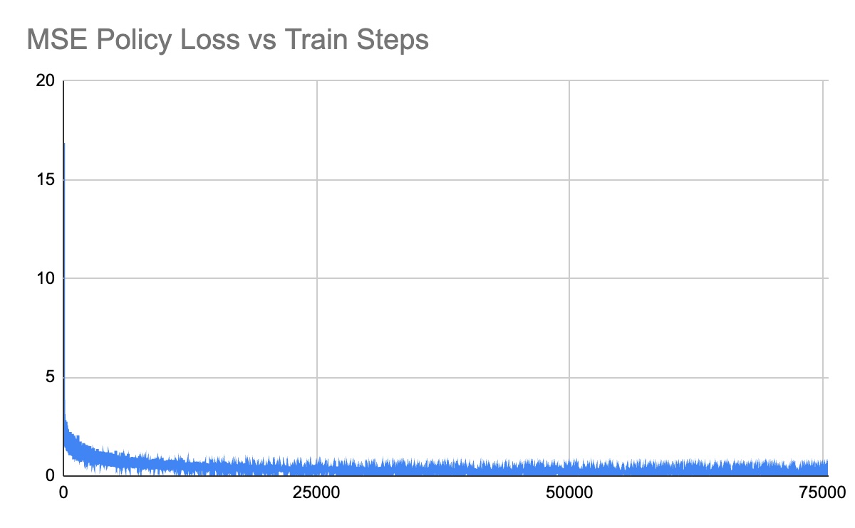
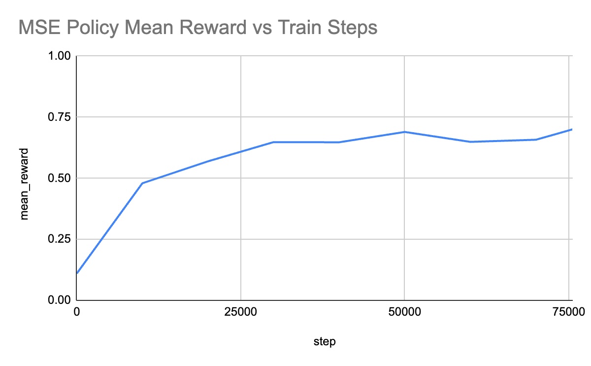
Performance Videos
| Before Training | After Training |
|---|---|
Flow Matching Policy Results
Training Curves
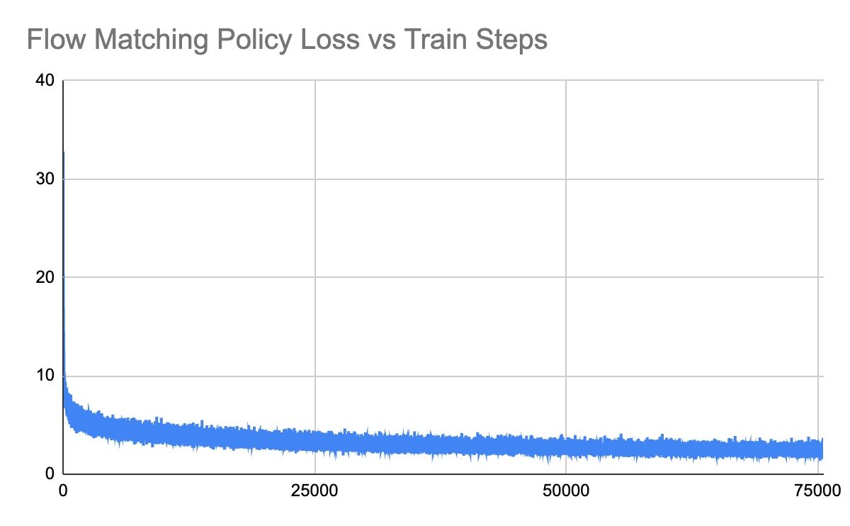
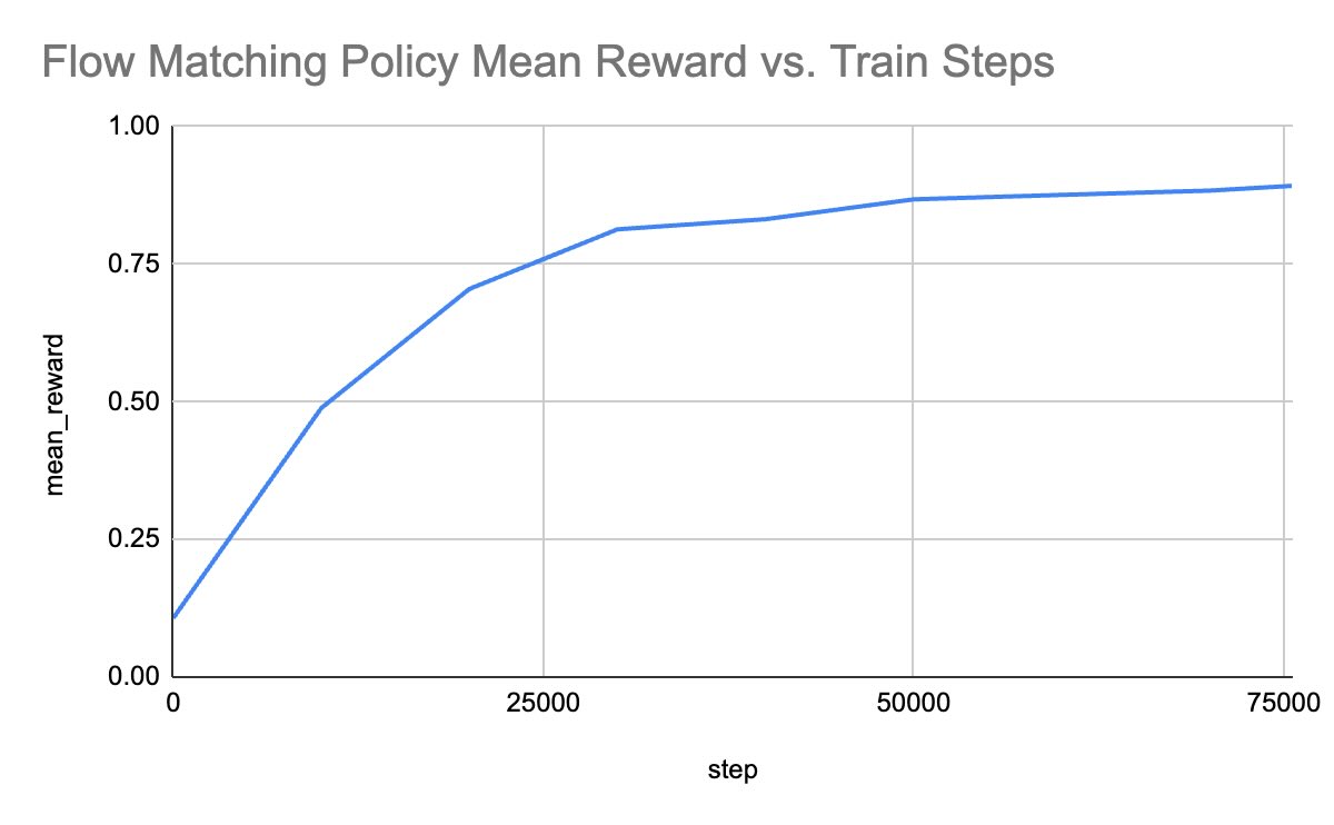
Performance Videos
| Before Training | After Training |
|---|---|
Qualitative Comparison
Qualitatively, we observe several key differences between the MSE and Flow Matching policies in the Push-T environment:
- Initialization and Early Training: At the start of training, the flow matching policy appears “jittery” and erratic. This is because it is sampling from a noise distribution and the vector field is not yet well-defined. In contrast, the untrained MSE policy tends to output a mean action that often results in the agent staying static or moving in an unhelpful direction.
- Final Performance: By the end of training, the flow matching policy significantly outperforms the MSE policy. The flow matching agent demonstrates clearer evidence of “planning”. It (re-)orients itself correctly relative to the T-block and makes purposeful pushes toward the goal.
- The “Mean Action” Problem: The performance gap is likely due to the training objective. An MSE policy learns to predict the average expert action for a given state. In multimodal scenarios (e.g., if an expert sometimes goes left and sometimes goes right to push the block), the MSE policy will predict the average, which may be straight into the block—leading to suboptimal behavior. Flow matching, being a generative model, can represent these multiple modes effectively, allowing it to “commit” to one valid path.
Conclusion
This assignment was fun. My next steps are to train policies for harder environments than Push-T, which will naturally necessitate the use of techniques more sophisticated than mere imitation learning. More on that coming soon!